

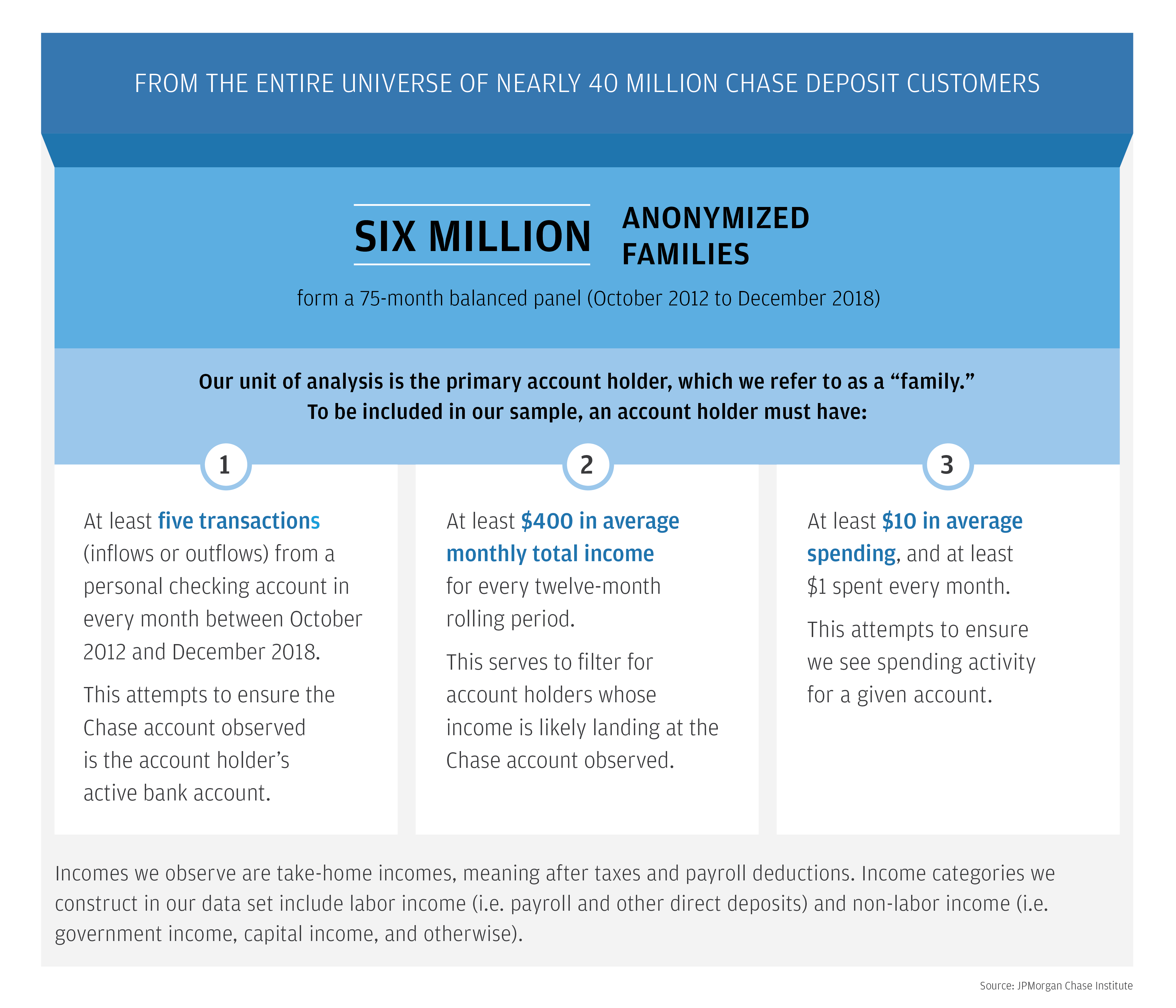
Source: JPMorgan Chase Institute
Latest news

An Ohio-based company is protecting first responders around the world
With support from JPMorganChase, Fire-Dex is providing protective equipment to firefighters in 100 countries and all 50 states.
Learn moreLatest news

Veteran’s Unconventional Path to Landing her Dream Job in Tech
U.S. Army Veteran Ashley Wigfall transitioned to a civilian role and charted her path to technologist through mentorship and skills training at the JPMorgan Chase tech hub in Plano, Texas.
Learn more
Research
A Monthly Stress Test to Guide Savings
October 23, 2019
Findings
In this report, the JPMorgan Chase Institute uses administrative bank account data to measure income and spending volatility and the minimum levels of cash buffer families need to weather adverse income and spending shocks.
Inconsistent or unpredictable swings in families’ income and expenses make it difficult to plan spending, pay down debt, or determine how much to save. Managing these swings, or volatility, is increasingly acknowledged as an important component of American families’ financial security. In prior JPMorgan Chase Institute (JPMCI) research, we have documented the high levels of income and expense volatility families experience. In this report, we make further progress toward understanding how volatility affects families and what levels of cash buffer they need to weather adverse income and spending shocks. We explore six key questions:
Source: JPMorgan Chase Institute
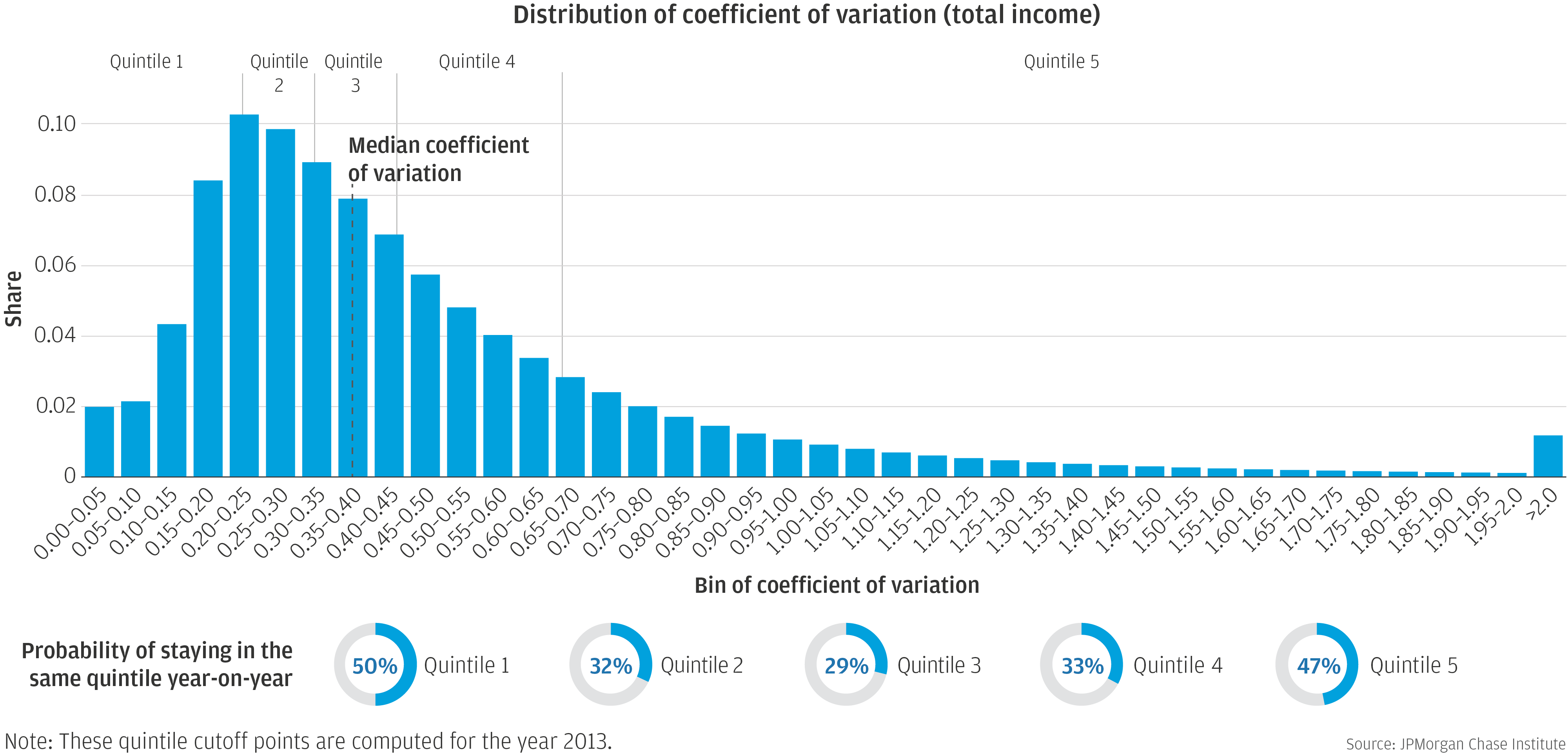
Income volatility remained relatively constant between 2013 and 2018. Those with the median level of volatility, on average, experienced a 36 percent change in income month-to-month during the prior year.
Source: JPMorgan Chase Institute
There is wide variation in the levels of income volatility families experience, both across families at a given point in time and also for a given family across time.
Source: JPMorgan Chase Institute
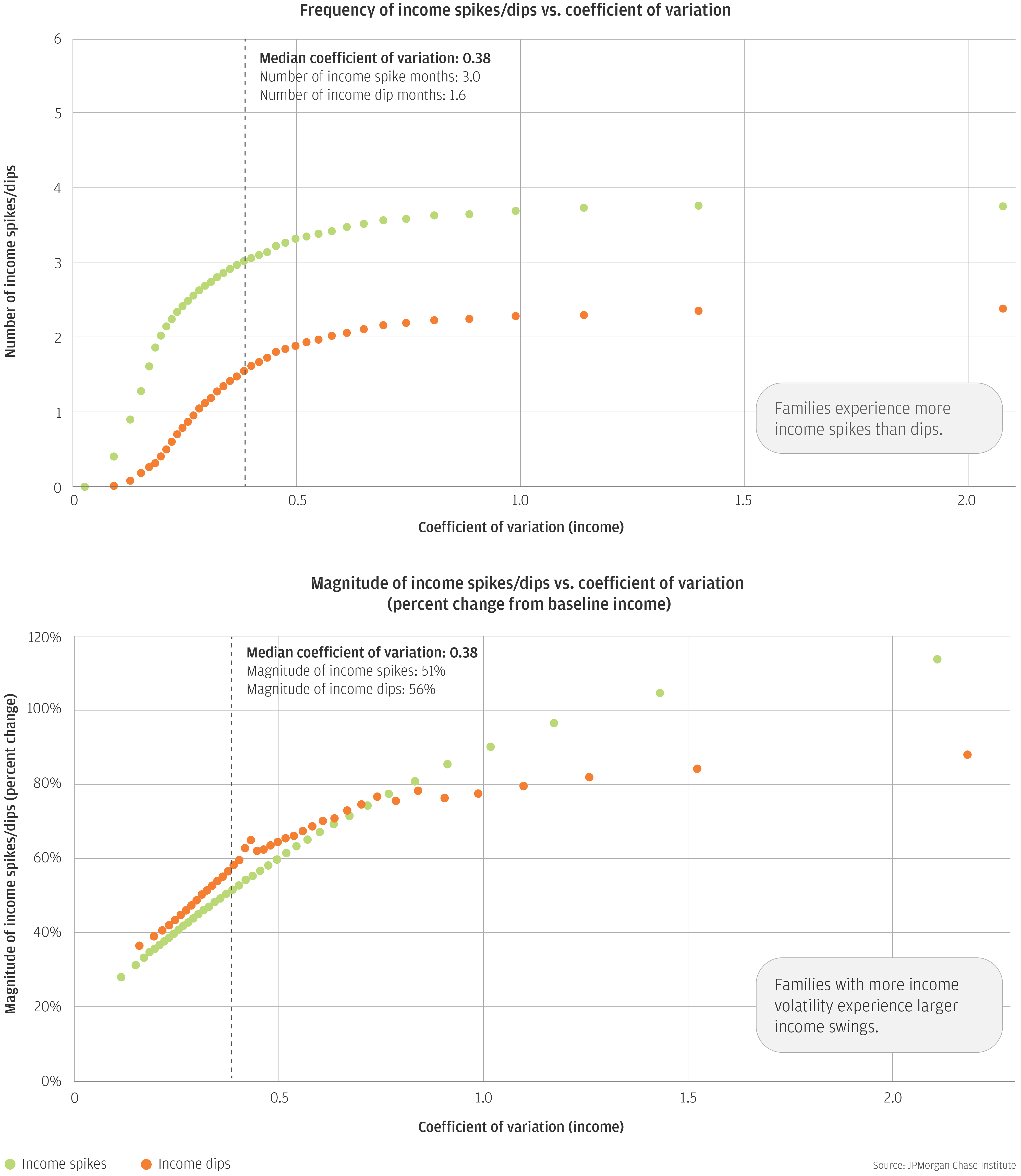
On average, families experience large income swings, in almost five months out of a year. Income spikes are twice as likely as income dips and most common in March and December. Families with the most volatile incomes experience swings that are larger but not more frequent than families with less volatile incomes.
Source: JPMorgan Chase Institute
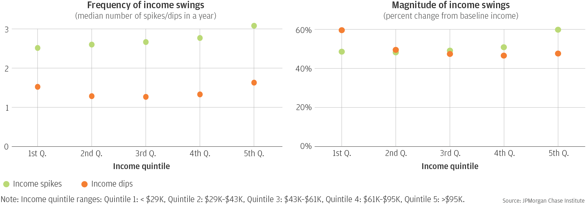
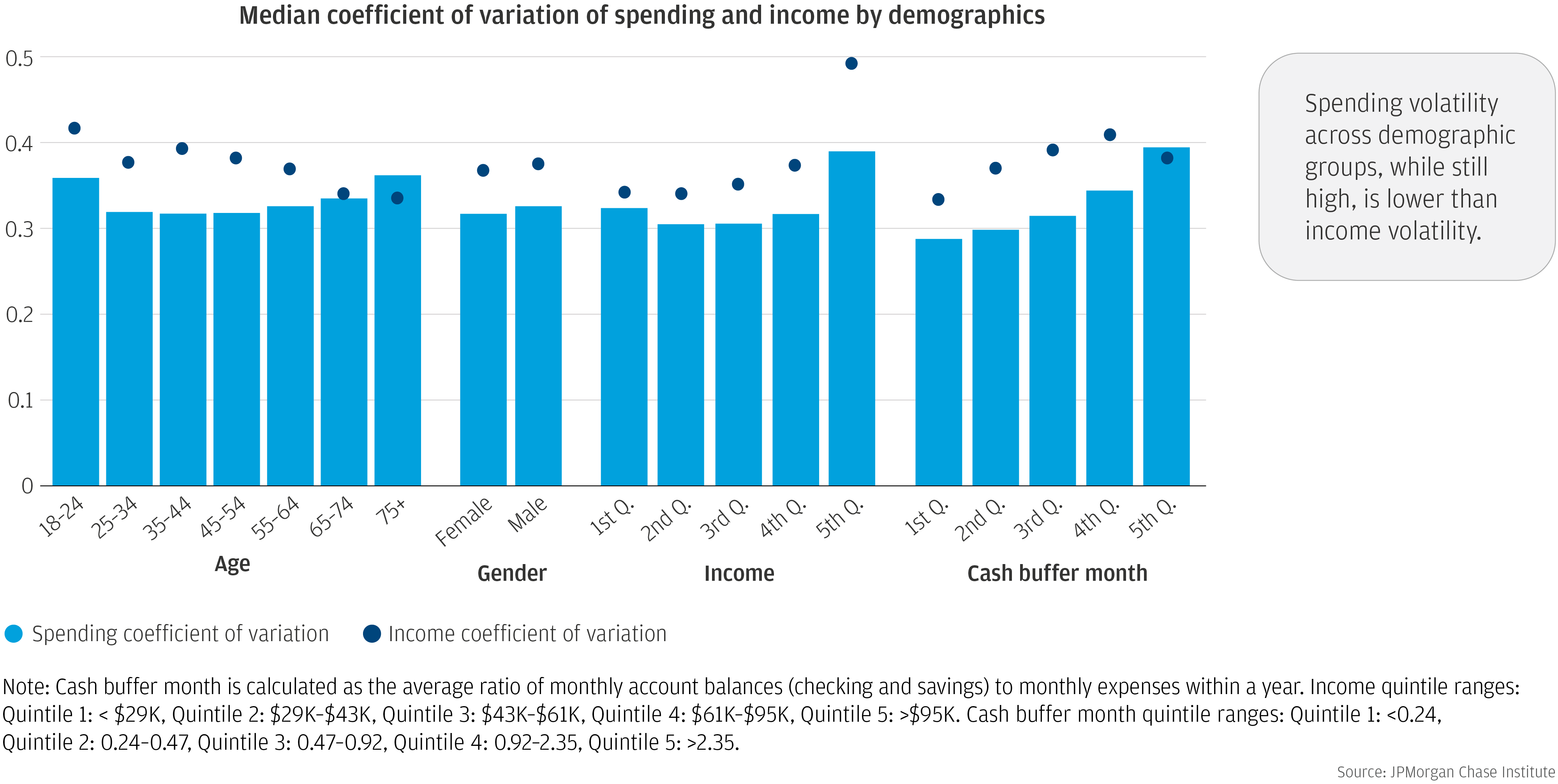
Income volatility is greatest amongst the young and the high income. However, downside risks, as measured by the magnitude and frequency of income dips, are greatest among low-income families.
Source: JPMorgan Chase Institute
The trend of spending volatility was flat between 2013 and 2018. While the level of spending volatility was also high, it was 15 percent lower than that of income volatility, except among account holders over the age of 75 and those with the largest cash buffers.
Source: JPMorgan Chase Institute
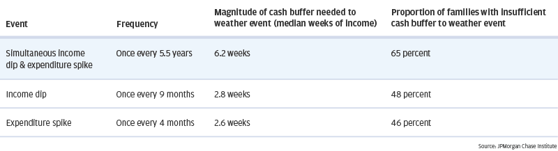
Families need roughly six weeks of take-home income in liquid assets to weather a simultaneous income dip and expenditure spike. Sixty-five percent of families lack a sufficient cash buffer to do so.
Our findings have important implications for designing savings strategies to improve families’ financial health and resilience. They suggest that the tools currently available to help families weather volatile income and spending could be better tailored to an individual’s cash flows. Simply saving a certain percentage of monthly income may leave a family with an inadequate cash buffer, exacerbating financial distress in cash flow negative months and resulting in under-saving during cash flow positive months. Instead, families may need to more aggressively harvest savings opportunities during income spike months. We provide empirical guidance for families, financial health advocates, financial advisors, and policymakers on the minimum levels of cash buffer families need to weather adverse shocks. Given the key role stability plays in the health of families’ financial life, it is critical that we continue to gauge how income and spending volatility are changing for American families and the implications for families’ financial health.
Authors

Chenxi Yu
Data Scientist

Diana Farrell
Founding and Former President & CEO

Fiona Greig
Former Co-President