

Figure 1: Advanced CTC payments boosted monthly income by 10 percent for the lowest-earning recipients.
Latest news

An Ohio-based company is protecting first responders around the world
With support from JPMorganChase, Fire-Dex is providing protective equipment to firefighters in 100 countries and all 50 states.
Learn moreLatest news

Veteran’s Unconventional Path to Landing her Dream Job in Tech
U.S. Army Veteran Ashley Wigfall transitioned to a civilian role and charted her path to technologist through mentorship and skills training at the JPMorgan Chase tech hub in Plano, Texas.
Learn more
Findings
On March 11, 2021, President Biden signed the American Rescue Plan Act of 2021 (ARPA) into law. The stimulus bill aimed to deliver direct relief to families and workers continuing to struggle financially during the ongoing COVID-19 pandemic. ARPA included provisions for an additional round of economic impact payments (EIP), state and local fiscal recovery funds, homeowner and rental assistance funds, and programs to help small businesses and unemployed workers.1 A notable component of ARPA was the expansion of the existing Child Tax Credit (CTC) program. Among other things, this expansion introduced automatically disbursed cash payments to the overwhelming majority of families with children under 17. It was both novel in its structure and unprecedented in its scale—characterized by its designers as “the largest child tax credit ever and historic relief to the most working families ever." Accordingly, the program provides a unique opportunity for policymakers to understand how effective future policies like the CTC might be.
Other studies have tried to measure the impact of the CTC expansion on household finances, particularly the impact of the expansion on household consumption. Studies leveraging data from the Census Bureau’s Household Pulse Survey show that recipients report using these advanced payments to pay for bills and other living expenses and establish differences in spending patterns by income and race (Pilkauskas and Cooney 2021; Karpman et al. 2021; Pilkauskas et al. 2022). However, these studies are not able to quantify how much of the advanced CTC payments households spent—a critical question for policymakers concerned with balancing the goal of increasing the welfare of families with children against concerns about potential adverse inflationary or labor market effects of expansions to CTC.2
This report seeks to fill this gap by using transaction-level data to estimate the impact of these accelerated payments on household spending. We explore a range of spending categories, including spending on durable goods, services, and debt payments. We also analyze whether spending responses differed by type of household—whether changes were more pronounced for lower liquidity households, or households of different races. Given the unprecedented nature of this program, ongoing assessments of the credits’ impacts on household finances will be important in understanding the program’s success and planning similar programs in future.3
ARPA introduced several specific updates to the Child Tax Credit. The credit amount was increased from $2,000 to $3,600 for children under age 6 and to $3,000 for other eligible children; eligibility was expanded to include 17 year-olds; the credit became fully refundable; and 50 percent of the credit was scheduled for automatic disbursal via monthly payments between July and December 2021. Families were automatically enrolled in the advanced CTC payments and the IRS provided a channel to opt out of advanced CTC payments for families that preferred to receive the full tax credit when filing their 2021 tax returns.4 Married couples with income up to $150,000 (or $112,500 for single parents) were eligible for the full credit; married couples with income under $400,000 (or $200,000 for single parents) qualified for at least $2,000 of the CTC, with $166 per child each month disbursed via advanced payments.
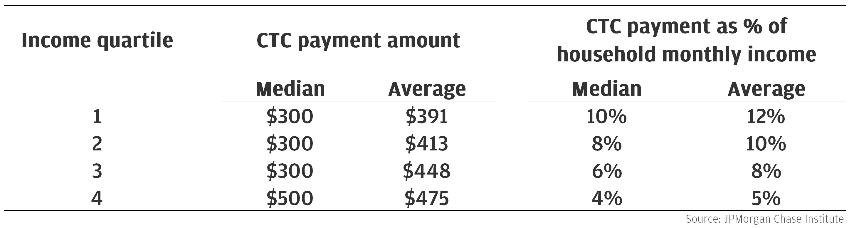
Advanced CTC payments substantially increased the income of families that received them—particularly lower income families. Among the recipients in our sample, the median household received $300 per month for households earning less than $73,000 in annual take-home income (the lowest three income quartiles; refer to the appendix for income quartile details), and $500 per month for households earning above that threshold (Figure 1). This difference is due to differing family composition across the income groups. Only 38 percent of the lowest-earning CTC recipients had more than one dependent child, compared to 61 percent of the highest-earning recipients (46 and 53 percent for the middle quartiles, respectively).5 Despite receiving, on average, greater monthly amounts, the overall income impact was lowest for the highest-earning households, whose monthly income increased by only 4 percent with the CTC payments. By contrast, the advanced CTC payments represented a 10 percent increase in monthly income for the lowest-earning households (those with annual take-home income less than $31,000). So while lower-earning households typically received lower payment amounts (due to the presence of fewer children per household), that amount had a greater impact on monthly income and may have therefore been felt more keenly.
Figure 1: Advanced CTC payments boosted monthly income by 10 percent for the lowest-earning recipients.
To understand the impact of advanced CTC payments on household consumption, we begin by comparing the spending behavior of CTC recipient households to the behavior of non-recipient households. To isolate the effect of the CTC payments themselves, we control for household-level differences in spending levels, as well as trends in spending levels over time that are common to both groups (see appendix for details). After removing these trends, we suppose that the spending behavior of non-recipients is similar to what recipients would have done had they not received the CTC payments.
Figure 2 shows how total spending of CTC recipients evolved week-to-week, relative to non-recipients. This can be thought of as “excess” spending among CTC recipients relative to non-recipients and is measured as a fraction of the household’s CTC payment: if a household received a $200 CTC payment and then spent $100 more than it would have otherwise, its excess spending in Figure 2 would be 0.5. Our measure of spending here is the sum of all payments made from each household’s accounts via debit card, paper checks, cash withdrawals, electronic payments, and Chase credit cards, excluding debt payments.6
We see a clear spending response after every advanced CTC payment (Figure 2). We also observe a downward sloping trend, indicating that apart from the spending spikes after each CTC payment, recipient households generally decreased their spending relative to non-recipient households in the months after the first CTC payment. This might be because CTC-recipients are more likely to be households with children who received larger EIP amounts in March 2021 and their spending is decelerating after that influx of cash, or some other behavior specific to households with children. It may also be that the large spending response after each payment is pulling some future spending forward in time. In the appendix, we present evidence that suggests that the former explanation—differing trends between households with and without children—is more likely.
Figure 2: CTC recipients’ spending spiked in each week of advanced CTC payments.
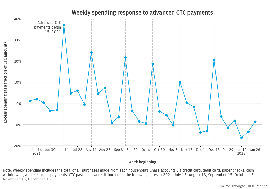
We can also use Figure 2 to calculate the marginal propensity to consume (MPC) out of CTC payments. This is how much of the average CTC payment was spent within the first week after receipt. Because of the observed downward trend in spending among CTC households, we measure the MPC for each payment by comparing the CTC recipients’ excess spending in the week the payment was received to their excess spending in the prior week. That is, the MPC out of the July 14 payment is the difference between the dot in Figure 2 for July 14 and the dot for July 7.
Using this approach, we calculate a 40 percent MPC for the first advanced CTC payment in July (Figure 3). In other words, within the first week of receipt, households consumed 40 percent of their CTC payment via spending on credit and debit cards, checks, cash, and electronic payments.
Figure 3: Recipients spent 40 percent of their July advanced CTC payments in the first week.
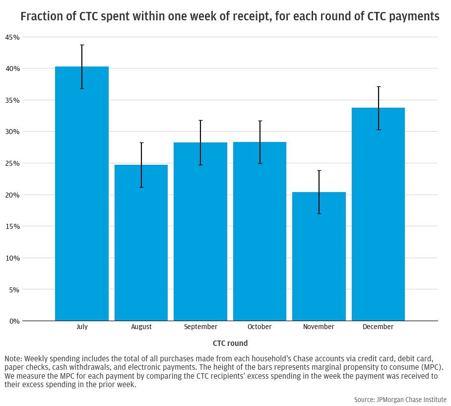
Beyond the July payments, we observe spending MPC values ranging between 21 percent (November) and 33 percent (December) for the advanced CTC payments.7 However, it is difficult to conceptualize marginal propensity to consume in a situation of monthly cash disbursals, particularly beyond the first month of the series. CTC payments land every month and are not (on average) fully consumed each month, meaning that household cash-on-hand in a given month is impacted by the amount of CTC payment and associated MPC from the previous month. It is therefore difficult to assess a marginal propensity to consume in the latter months of the advanced CTC payment series. For clarity of concept and measurement, this report will focus results on MPC measurements out of the July advanced CTC payments.
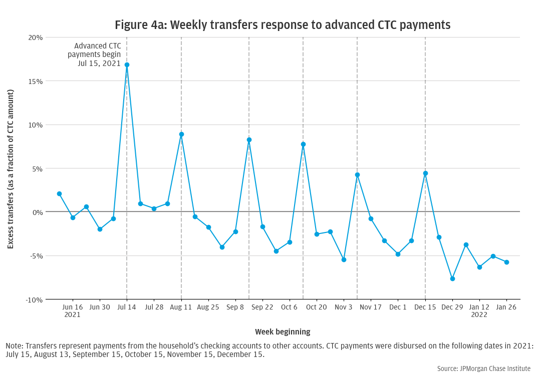
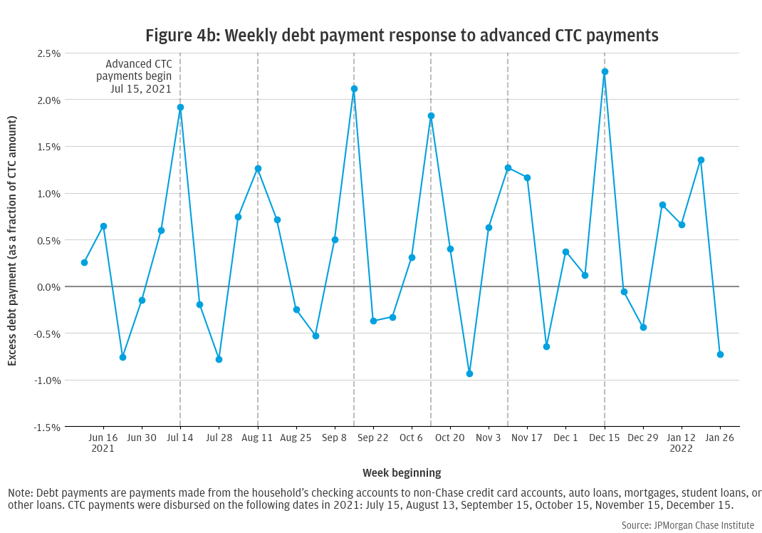
Like with spending, we also observe that advanced CTC recipient households respond to the CTC payments by transferring more cash to other accounts than non-recipient households do. The accounts receiving these transfers could be owned by the household—such as savings accounts or non-Chase accounts—or accounts owned by other households, such as family members. CTC recipient households in our sample transferred 18 percent of their July CTC payments to other accounts (Figure 4a). Debt payments—to non-Chase credit cards, auto loans, mortgages, student loans, or other loans—were much less responsive to advanced CTC payments than spending or transfers. While debt payments exhibit clear response patterns during CTC weeks (Figure 4b), only 1 percent of July CTC dollars go toward debt payments.
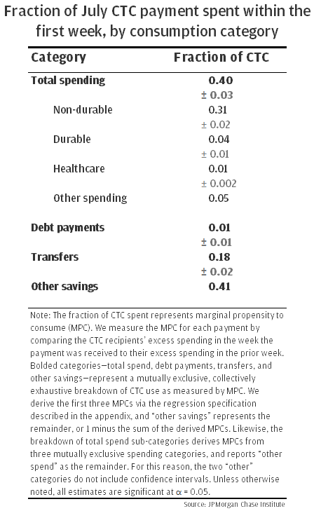
Finally, we differentiate types of spending within the total spending category (Figure 5). Most spending out of CTC payments goes toward non-durable goods, which accounts for more than three quarters of the total spending response (31 percent of the CTC payment).8 Of that non-durable spending, roughly 12 percent goes toward groceries and fuel (or 4 percent of the CTC payment). Durable goods also exhibit a clear spending response during CTC payment weeks, but at notably lower levels (4 percent of CTC amount).9 Healthcare spending also increases with CTC receipt, but while the increase is statistically significant, it small in magnitude (approximately 0.5 percent of CTC amount).10
Overall, households consumed 40 percent of July CTC payments via spending within one week of receipt, with the majority of that spending on non-durable goods; an additional 18 percent went toward transfers to other accounts, with most of the remainder held as cash savings in households’ checking accounts.
Figure 5: Recipients spent 40 percent of July CTC payments in the first week, transferred 18 percent to other accounts, and maintained most of the remainder as cash savings.
Compared to households with substantial liquidity, cash-constrained households are more likely to cut spending upon job loss, or increase spending after receiving a tax refund (e.g. Farrell et al. 2019). To assess the sensitivity of the CTC spending response to liquidity, we compare the marginal propensity to consume of high liquidity families to that of low families. We measure the liquidity of a household by computing its cash buffer—the amount of cash it has on hand divided by its typical spending. By this metric, families with smaller cash buffers are more liquidity constrained (see the appendix for details on the construction of our cash buffer metric, as well as how cash buffer compares with income).
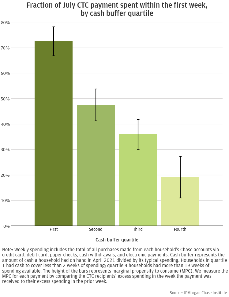
We find that the spending response to advanced CTC payments among low-liquidity households is significantly stronger than it is among high-liquidity households. We observe clear spending responses during CTC payment weeks across all cash buffer quartiles, though the level becomes more muted for higher buffer groups (Figure 6). Households in the lowest cash buffer quartile (with cash-on-hand covering less than 2 weeks of spending) consumed 73 percent of their July CTC payments via spending in the first week (Figure 7). By contrast, households in the highest cash buffer quartile (with cash-on-hand covering over 4 months of spending) consumed only 19 percent of their CTC payments via spending in the first week. Although the spending response decreases for each increase in cash buffer quartile, the households with the most cash-on-hand still spent a non-trivial fraction of the CTC payment in the first week.
Figure 6: CTC recipients’ spending spiked in each week of advanced CTC payments, much more so for low-liquidity recipients than their high-liquidity counterparts.
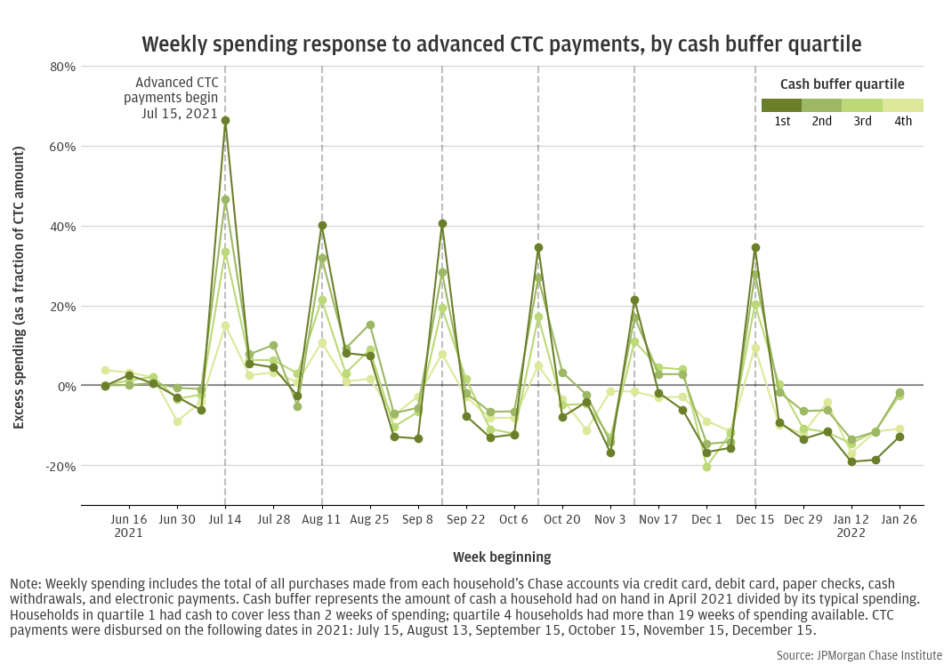
Figure 7: Recipients with the lowest liquidity spent 73 percent of their July CTC payments in the first week, compared to only 19 percent spent by the highest liquidity recipients.
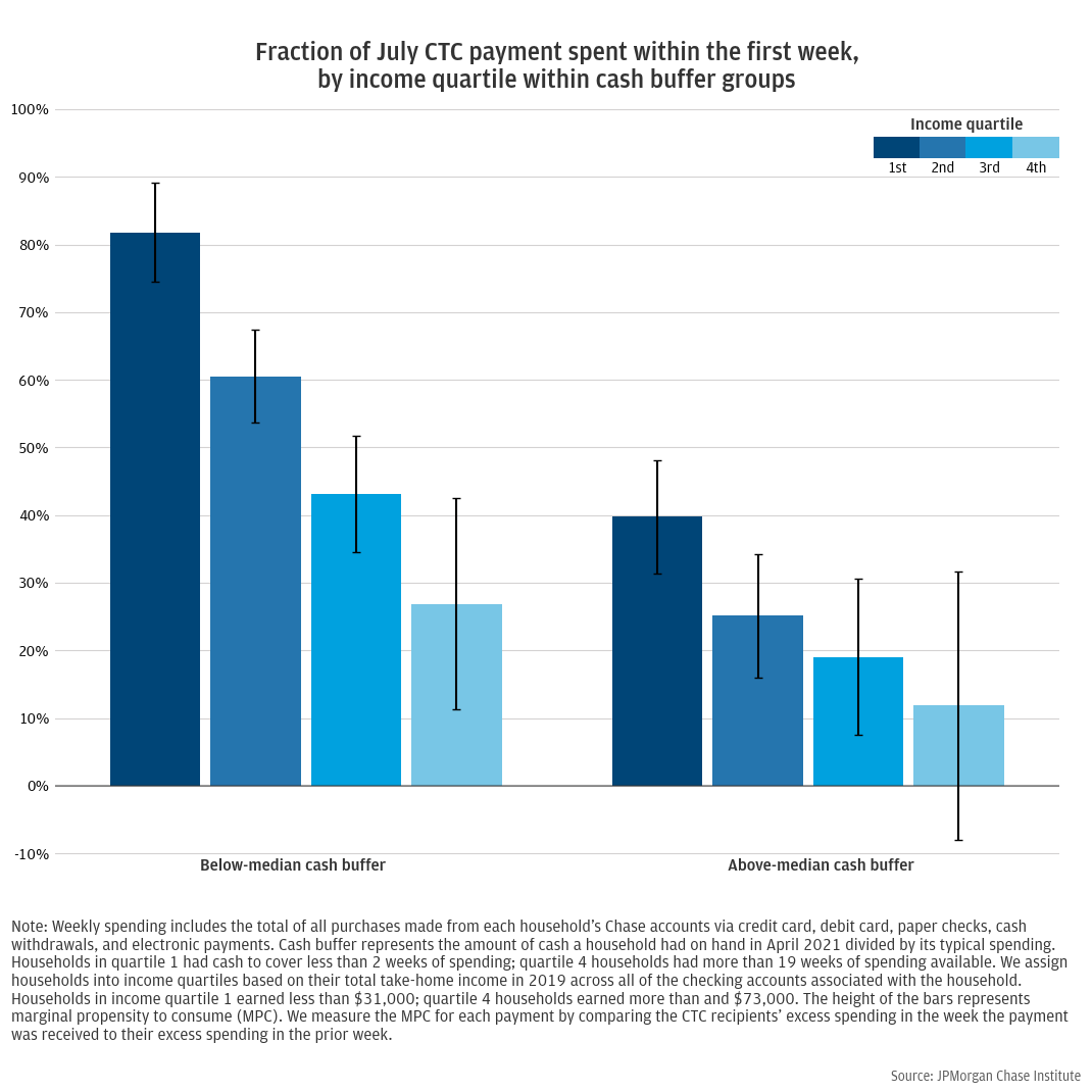
Households’ cash-on-hand remains a strong predictor of spending response even when we account for household income (Figure 8). Among households with below-median cash buffers, the spending response was strongest for the lowest earners, but still notable for high-earning households, indicating that cash liquidity was a stronger predictor of spending response than income. The lowest earners (take-home income under $31,000) in this group spent a substantial share—80 percent—of July advanced CTC payments within the first week. The highest earners (take-home incomes greater than $73,000) still spent nearly 30 percent within a week.
Figure 8: Of recipients with below-median liquidity, the lowest-income households spent 80 percent of their July CTC payments in the first week, and the highest-income households still spent nearly 30 percent.
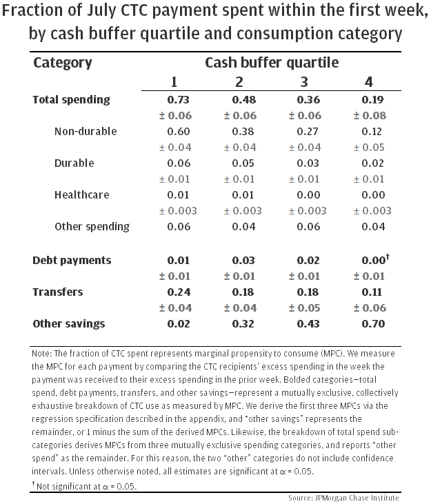
As with our analysis of the overall sample, we again break down consumption of advanced CTC payments across a set of categories, and assess how cash buffer differences contribute to trends in how households distribute their consumption across these categories (Figure 9). Within each cash buffer quartile, the relative size of the spending response by consumption category mirrors the overall results in Figure 5. Among active uses of CTC money—the categories listed above “other savings”—the majority went toward spending on goods and services, especially non-durable goods, and the next most common use was transfers to other accounts.
Households with lower cash buffers actively used a greater share of their CTC money, relative to households with higher cash buffers. That is, households with low cash buffers used a larger portion of their CTC payments via spending and debt payments, maintaining very little “unused” CTC money (2 percent, vs. 70 percent for high-buffer households). While this “other savings” bucket represents additional cash savings in the household’s accounts, it also demonstrates a lack of active engagement with the received funds. High-liquidity households appear especially unresponsive to advanced CTC payments. They not only consume less of their CTC via spending relative to low-buffer households (19 percent vs. 73 percent), but also make proportionally smaller debt payments and transfers to other accounts.
Figure 9: Low-liquidity recipients consumed a larger portion of their July CTC payments via spending and debt payments, and maintained very little as cash savings (2 percent vs. 70 percent for high-liquidity recipients).
Previous JPMorgan Chase Institute research has documented racial gaps in various financial outcomes. In particular, the Institute observed large racial differences not only in income, but also in liquid assets, which we have just shown to be a key driver of CTC consumption response. While existing research has assessed racial differences in CTC response (e.g., Karpman et al. 2021), our data uniquely positions us to add to this conversation given our ability to observe both race and liquidity to further contextualize observed differences by race.
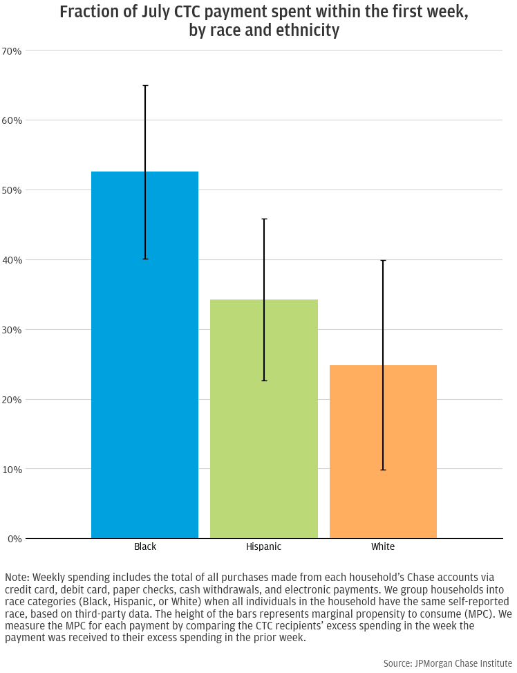
Analyzing the subset of households for whom we have self-reported race information (see appendix), Black households have the highest spending response, spending about half of CTC payments within the first week (Figure 11). The response was lower for Hispanic and White households, with White households having the smallest response. However, while the difference in these responses is large in an economic sense, we cannot statistically distinguish the spending responses of Hispanic households and White households (the p-value of a Wald test of these parameters is 0.33).11
Figure 10: CTC recipients’ spending spiked in each week of advanced CTC payments, with higher July spending responses for Black and Hispanic recipients than their White counterparts.
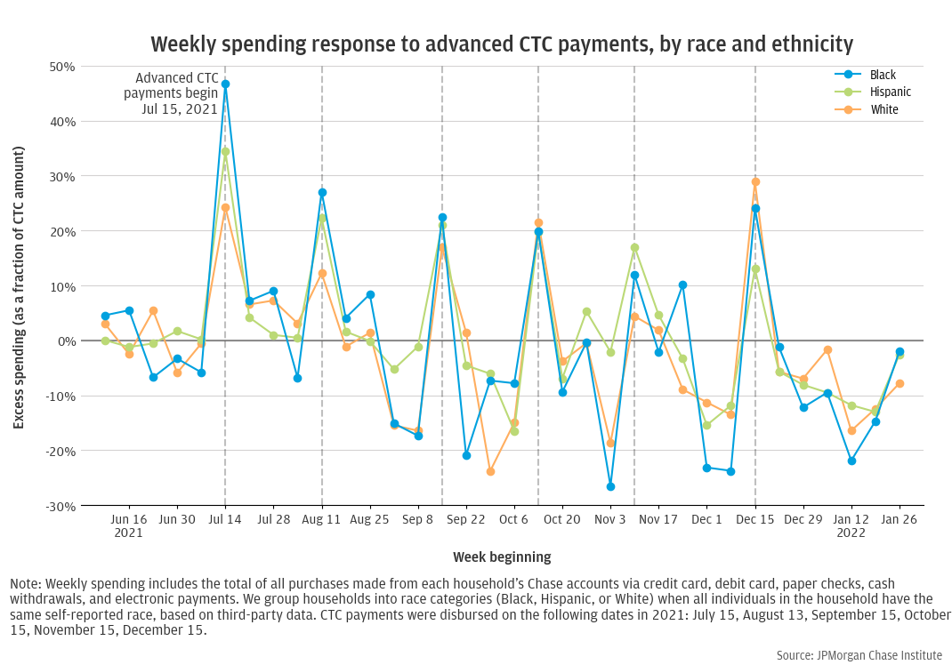
Figure 11: Black recipients spent 53 percent of their July CTC payments in the first week, compared to 34 percent for Hispanic and 25 percent for White recipients (though Hispanic-White differences are not significant).
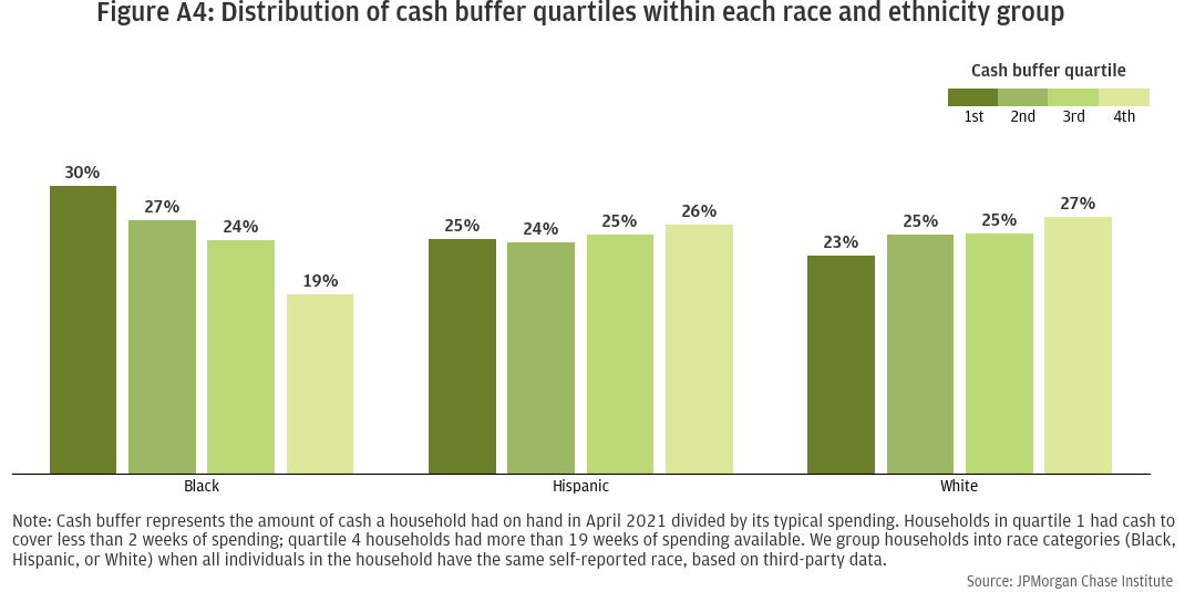
We next assess how much of the differences in spending response across race groups may be driven by other underlying differences across the groups. For example, households’ cash buffers differ significantly by race: 30 percent of Black households have a cash buffer in the lowest quartile of the population, compared to only 23 percent of White and 20 percent of Hispanic households (see appendix, Figure A4).
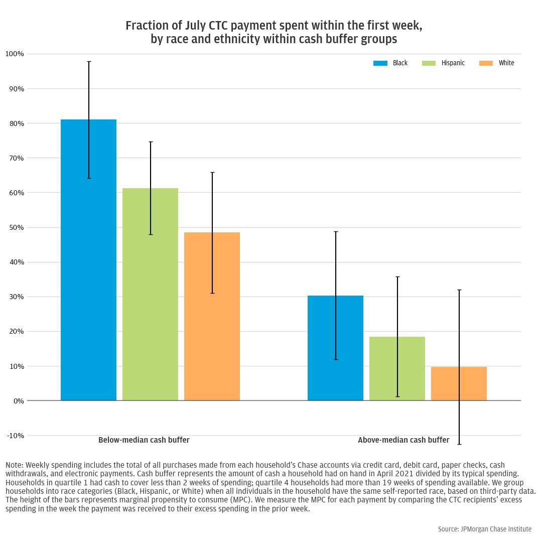
The differences in spending response by race are partially explained by differences in cash buffers (Figure 12). For households with above-median cash buffers, differences in spending response by race are no longer statistically significant. Large standard errors result in wide confidence intervals, and an MPC that is not statistically distinguishable from zero for White households. For households with below-median cash buffers, Black households spent the largest share of their July CTC payments within one week (81 percent) followed by Hispanic and White families (61 and 48 percent, respectively). As in the aggregate results above, differences between White and Hispanic households are not statistically significant. However, the response of Black households is still significantly different from that of White households (p-value 0.009) and marginally significant compared to Hispanic households (p-value 0.073).
This remaining difference is likely driven by several factors. First, even among households with below-median cash buffers, there are still differences across race groups in cash-on-hand. Appendix Figure A4 shows that among below-median households, Black households are relatively more likely to be in the first quartile. Second, other financial characteristics affect the CTC response as well; as we show in Figure 8, income still affects the spending response even after conditioning on liquidity. Finally, there may be other race-specific factors not captured by income or cash buffer that affect the CTC spending response, such as differences in familial or intergeneration wealth (Farrell et al. 2020).
Figure 12: Racial differences in spending responses to July CTC payments are substantially smaller among households with similar liquidity.
Implications
Families with children may spend substantial shares of payments from programs like the Advanced Child Tax Credit. Across groups, we found that advanced CTC recipients spent 40 percent of their July CTC payments, the majority of which went to non-durable goods. Notably, many of these families were already holding unusually high cash balances due to Economic Impact Payments. Given the sensitivity of the consumption response to cash liquidity, it is possible that families would spend an even higher share of future payments in the context of household liquidity closer to historical levels.
To reach families that are most likely to utilize the payments, policymakers might consider programs that target families that are low-liquidity in addition to being low-income. We found that low-liquidity families were significantly more likely to spend out of advanced CTC payments than were high-liquidity families. Cash liquidity was a very strong predictor of spending response. Recipients with the lowest liquidity—deposit account balances totaling 2 weeks of spending or less—spent 72 percent of their July CTC payments. Moreover, they actively engaged with most of their July CTC payments, maintaining only 2 percent as cash in the checking account. Income did differentiate consumption responses among low-liquidity families. Low-income recipients with below-median liquidity had the strongest response of any group, spending 80 percent of their July CTC payments within one week. While high-income recipients exhibited a notably strong spending response when they had below-median liquidity, they spent just under 30 percent of this first payments over the same week.
High-liquidity families were notably unresponsive to advanced CTC payments. In contrast to low-liquidity families, recipients with the highest liquidity—who had nearly 5 months of typical spending in their deposit accounts—actively engaged with only 30 percent of July payments, leaving the remaining 70 percent of the payment untouched in their checking accounts. These families only transferred 2 percent of July CTC payments to other accounts, while low-liquidity families transferred 18 percent. While we characterize both transfers and cash left in checking accounts as forms of savings, transfers reflect a more active response to a payment.
The spending response to a similar future program is likely to be larger than what we find here because cash balances were historically high in 2021 due to the pandemic. As recent Institute work has shown, cash balances were elevated in the second half of 2021 when advanced CTC payments landed. This was especially true for lower-income families and younger families. Given our finding that families respond less to CTC payments when they have high cash buffers, similar initiatives are likely to see higher spending responses if they occur when cash buffers are no longer generally elevated.
Underlying differences in liquidity are also largely responsible for observed aggregate differences in consumption response by race. The consumption response to advanced CTC payments differed by race and ethnicity, with Black families spending a larger proportion of their July payments within the first week than Hispanic and White families (the latter two of which did not significantly differ). However, after accounting for differences in household liquidity, racial differences in spending responses to July CTC payments for high-liquidity households were substantially smaller. This again underscores the importance of accounting for liquidity in targeting future cash disbursal initiatives.
Our sample covers 2.4 million households whose members were active checking account users between January 2019 and January 2022. We apply several filters to the broader set of JPMorgan Chase account holders to arrive at this sample of 2.4 million households. To ensure representative households, we remove those with demographic outliers (extreme values for age or number of household members). To ensure that a household uses their JPMC accounts as primary financial vehicles, we require the presence of JPMC deposit accounts (not just credit cards), require minimum activity of 5 transactions per month, and require minimum income of $12,000 for every year 2019 through 2020. Finally, to ensure to ensure visibility into most of the household’s spending behavior via their JPMC checking and credit card accounts, we limit to households with relatively small (if any) monthly credit card payments to other banks. We also exclude families that did not receive Economic Impact Payments (EIP) in both 2020 and 2021. The income eligibility threshold for EIP—$150,000 for joint filers or $75,000 for individual filers—is lower than the eligibility threshold for advanced CTC payments, therefore our sample consists of households that are eligible to receive the full CTC amount.
We classify households as CTC recipients or non-recipients based on the presence and frequency of CTC payments into their deposit accounts. Our sample contains approximately 460,000 CTC recipient households which received all six rounds of CTC payments via ACH deposits into their accounts between July and December 2021. An additional 1.4 million households are classified as CTC non-recipients based on receiving no advanced CTC payments. The remaining 526,000 households are excluded from analysis, as we cannot confidently determine CTC receipt during the disbursal period. Specifically, our CTC recipient group excludes households that received fewer than six monthly payments or who received inconsistent monthly CTC payment amounts, while our non-recipient group excludes families that received stimulus payments for one or more dependent children in 2020 or 2021. To ensure that our measures of CTC receipt and CTC amounts are accurate, both CTC recipient and non-recipient groups exclude a small share of families that may have received CTC payments in the form of paper checks, because we cannot verify the paper checks with as much certainty as ACH payments. We refer to the combined sample of 1.9 million CTC recipient and non-recipient households (after removing these indeterminate households) as our analysis sample. All results reported in this document are based on this analysis sample.
We observe households’ total income and spending across all their checking and credit card accounts from May 2021 to January 2022. We construct liquidity measures for each household based on the balances held in their checking and savings accounts, relative to their typical spending. See the below Measures section for details.
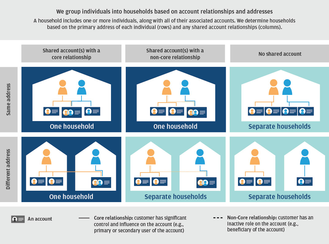
This report utilizes a new unit of analysis, which we refer to as a household. Households enable a comprehensive view into family demographics and finances by allowing us to understand the household composition across all members, as well as household finances across the full set of accounts associated with any household member.
A household can include one or more individuals, who share a core relationship on at least one of their accounts (e.g. they are primary or secondary account-holders on the same account). When analyzing household finances, we consider all accounts associated with each individual in the household.
Income: Measured as total household inflows (excluding transfer inflows) over calendar year 2019 across all of the checking accounts associated with the household. This is, by construction, a measurement of take-home income. As noted above, we remove households with insufficient income from our analysis sample. Household incomes must be at least $12,000 in 2019, 2020, and 2021 to be included in our data.
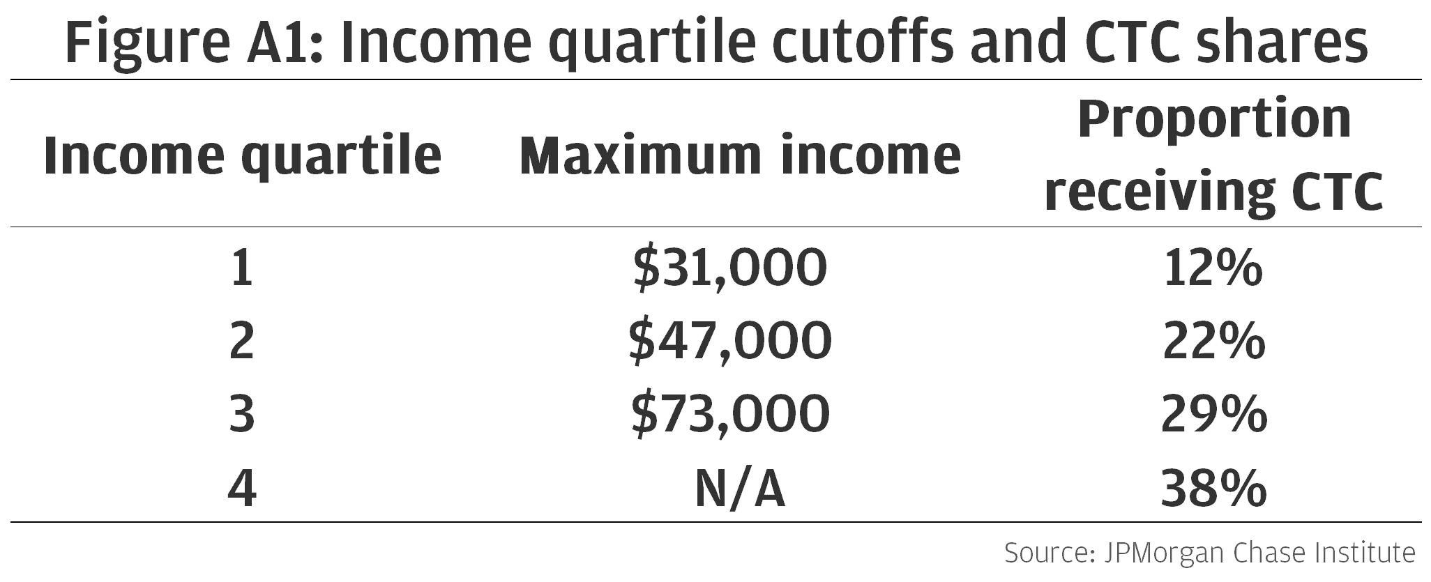
Income quartile: We assign households into income quartiles based on the income metric described above. Income quartiles are defined on the entire sample of households, after applying the filters described in the Data Asset section. This means that CTC recipients are not evenly distributed across income quartiles. See below for income cutoffs and the share of each quartile comprised of CTC recipients. Note that income cutoffs are slightly higher than in past Institute research because our household unit of analysis includes more accounts per household.
Figure A1: Income quartile cutoffs and CTC shares
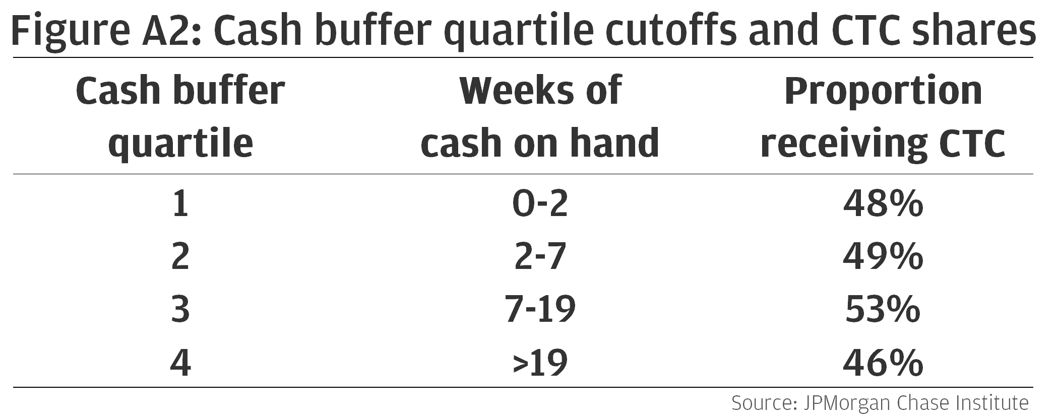
Cash buffer: A household’s cash buffer measures how long (in weeks) it would take for a household to deplete their cash balances at their typical spending rate. We construct cash buffers for a household by discounting the balance in their accounts by their typical weekly spending. Specifically, a household’s weekly cash buffer is the ratio of median weekly balance to median weekly spending.
Cash buffer quartile: We assign households into cash buffer quartiles based on their cash buffer in April 2021. See below for how many weeks of cash-on-hand each cash buffer quartile represents, and the share of each quartile comprised of CTC recipients.
Figure A2: Cash buffer quartile cutoffs and CTC shares
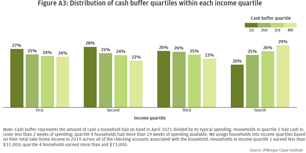
While cash buffer is somewhat correlated with income, they represent distinct concepts. Cash buffer measures how cash-constrained a household is relative to its own spending habits. High-income families often maintain low cash buffers in their checking and savings accounts (either due to higher spending habits than low-income families, or higher rates of transferring funds to other types of accounts). The reverse is also often true, with low-income families maintaining high cash buffers (likely due to having low levels of typical spending). Indeed, 20 percent of the lowest-earning households in our sample are in the highest cash buffer quartile, whereas 24 percent of the highest-earning households are in the lowest cash buffer quartile.
Figure A3: Distribution of cash buffer quartiles within each income quartile
Race: Household race is derived from the self-reported race of the individuals in the household. Individuals’ self-reported race metric comes from third-party data and is not available for every individual. Our analysis sample includes approximately 60,000 households that have self-identified race for all members of the household. We define a household as belonging to one of four broad race categories (Asian, Black, Hispanic, or White) when all individuals in the household have the same self-reported race; households with individuals who have two or more race categories are categorized as multi-race. Due to low coverage of certain self-reported race categories in our household sample, we exclude groups that had too few observations for analysis: Asian households and multi-race households.
Figure A4: Distribution of cash buffer quartiles within each race and ethnicity group
To estimate the effects of advanced CTC payments on consumption, we use a difference-in-differences research design. It is important to note, however, that this case is imperfectly structured for a traditional difference-in-differences analysis because we know that our two groups—recipients and non-recipients of advanced CTC payments—differ in other ways besides their CTC recipiency alone. In an ideal difference-in-differences design, pre- and post-policy outcomes for a treated group are compared to pre- and post-policy outcomes of a reference group that was not affected by the policy intervention but is otherwise similar to the treatment group (e.g. households on one side of a state border versus those just on the other side of the border). If the treatment and control groups are identical in all ways except for their receipt in treatment, then the control group may provide a credible counterfactual for the treatment group; that is, the treatment group likely would have behaved like the control group had they not been treated. In our case, implementation of the advanced CTC payments was nation-wide and affected all qualifying households that did not proactively opt out. This means that our “treatment” group of CTC recipients is comprised only of households that have dependent children, whereas our “control” group of non-recipients is comprised of households with none.12 In other words, our two comparison groups will be fundamentally different beyond the policy intervention and these differences in characteristics may lead to differences in behavior over time and the control group’s behavior may not be a counterfactual for the treatment group’s behavior. For this reason, we do not refer to these groups as “treatment” and “control” in this report.
We have made efforts to understand and quantify differences between recipient and non-recipient households and to account for those analytically wherever possible. Specifically, we include weights in our regression based on several key differentiating characteristics between the groups (details below). However, this is not sufficient to entirely remove differences between CTC recipients and non-recipients for a clear view of consumption differences that holds all else constant. Behavioral changes over time—which differ by group—create challenges to understanding consumption differences between recipients and non-recipients. (See detailed discussion and additional assessments in the box on Differing Trends by CTC Recipiency.)
Regression specification: We run regressions of the following form:
yit=αi+δt+βτCTCi1τ+εit
The dependent variable of interest for household i in week t is yit. See below for a full list of the dependent variables used in our analysis. Individual level fixed effects (αi) are at the household level, while time fixed effects (δt) are at the weekly frequency. CTCi represents the advanced CTC payment amount for household i. As noted in the Data Asset section, we remove from our sample the rare households that had inconsistent CTC payment amounts, therefore this CTCi is consistent at the household level across all six months of advanced payments. 1τ is an indicator (or dummy) variable for week τ where τ is only distinguished from t because t indexes all weeks in the sample while τ only includes weeks from June 9 and onward. (See Week variables below for additional discussion.) Weeks before June 9 establish the baseline difference between recipients and non-recipients. Thus, the βτ coefficients capture the change in the average difference in yit between CTC recipients and non-recipients in week τ relative to the difference in the baseline period. Furthermore, because CTCi is the dollar amount of CTC received, the unit of measurement of βτ is CTC amount itself; that is, βτ is the excess spending done by recipient households relative to non-recipients expressed as a fraction of the CTC payment the household received. Finally, εit represents the error term.
We also estimate similar specifications where the β and δ coefficients are allowed to vary by liquidity, income, and race groups, which allows us to measure separate CTC responses for each of these groups.13
As discussed below, we use analytic weights in each regression to account for underlying differences in household characteristics between CTC recipients and non-recipients. We also cluster standard errors at the household level.
Dependent variables: To assess a complete picture of household consumption, we study several dependent variables.
Prior to use in regression, we scale the dependent variable via a two-step process, to account for both seasonality and differing spending levels across households.
Scaled value in week t= ((2021 week t value)-(2019 week t value))/(2019 median weekly total spending)
Note that the scaling denominator is always based on total spending, for every dependent variable. This is due to the relative rare occurrence of some types if consumption, for example healthcare spending, which often has a weekly median of zero for typical households. So that βτ can still be interpreted as a fraction of CTC amount, we also scale the CTC amount in the same way.
Accounting for credit card spending: Note that credit cards show up in two of our dependent variables, total spending and debt payments. The distinction here is Chase vs. non-Chase cards. We can observe any spending charged to a Chase credit card at a granular, transaction-level data. We see the transaction date and category, and can therefore include these transactions alongside other weekly spending categories. On the other hand, we cannot see details of how customers use their non-Chase credit cards. We can only observe the presence of other credit cards when a payment is made from a household’s Chase account to the non-Chase card bill. We therefore classify these payment transactions as debt payments, since the spending occurred prior and the payment represents paying down the debt owed to the credit card. We do not count payments toward non-Chase credit card bills as spending, since we do not know when or how the spending occurred, nor how much of the payment covers older debts on the card. Likewise, we do not count payments toward Chase credit card bills as debt payments, as we have already included this activity in our spending metrics.
Week variables: As noted in the regression specification, the independent variables of interest are household-level CTC amount and weekly dummy variables. We construct custom week boundaries so that the CTC payment lands as early in the week as possible. This enables the best understanding of consumption response, as each CTC week will include several days of observed spending following the CTC payment. Unfortunately, CTC payments are not scheduled based on day of the week, but instead land on the 15th of every month (or the preceding business day, if the 15th is not a business day). The result is that three CTC payments land on Wednesdays or Thursdays (July, September, December), two land on Fridays (August, October), and one lands on a Monday (November). To maximize post-CTC days per week, we construct our weeks to run Wednesday through Tuesday. This means that for five of the six CTC payments, the week of payment allows us to observe the payment day plus the 4 to 6 following days. Because November’s CTC payments land on a Monday, we only observe CTC payment plus 1 following day. This results in low consumption response estimates for November, since response to the payment gets distributed across 2 weeks.
Our analysis sample includes weekly data for each household beginning 9 weeks prior to the first CTC payment, and continuing through the end of January 2022. The first four weeks (9 to 6 weeks before the first CTC, or May 12 through June 8) serve as a reference period, during which behavioral differences between recipient and non-recipient households are established. When plotting the impulse response (βτ ) we subtract the average of the βτ for June 9 through July 7 (those before the first CTC payment) from each point in the plot, to level-set the series.
Weights: When regressing, we apply weights to non-CTC-recipient households so their demographics mimic those of the CTC recipients on key dimensions that differentiate households with and without children. We include three factors in this weighting scheme:
We compute weights based on the joint distribution of these three variables, as observed in CTC recipient households.14 For a target proportion based on the joint distribution in the CTC recipient group, and an actual proportion based on the joint distribution in the non-recipient group, household-level weights for non-recipient households are calculated as:
Weight=(Target proportion)/(Actual proportion)
Modeling sample: Prior to performing regressions, we apply additional filters to our analysis sample. First, we randomly select just over 300,000 households in each group (CTC recipients and non-recipients) from the full sample to enable efficient computation of the regressions. We also remove households with extreme values of scaled CTC amount or the dependent variable of interest (i.e., households with near-zero median spending). Finally, we remove households with extreme values of our weighting variables, specifically households with more than two adults.
CTC recipient households are fundamentally different from non-recipient households in many ways and are therefore difficult to directly compare. Our regression approach was unable to fully isolate CTC effects from underlying differences in household type, despite weighting on several key differentiating factors: household maximum age, number of adults, and amount of cash buffer (see the appendix for details). Figure 2 illustrates this issue in its downward sloping trend, indicating that spending differences between CTC recipient and non-recipient households are not steady over time.
Previous Institute research has highlighted steeper balance trajectories for CTC recipient households in the months prior to the advanced CTC payments (see linked Figure 7). That report showed that CTC-recipient families had much higher balances than non-recipient families after the final EIP stimulus payments in March 2021 and depleted those balance gains over subsequent months. These balance trends indicate that CTC recipient families likely had different spending trajectories than non-recipient families in the months following the final stimulus payment, with CTC recipient spending declining relative to the non-recipient group over time. This relative deceleration of spending among the CTC recipients as they finish spending down their EIP money will be reflected in the estimated response to CTC receipt because “large EIP amount” is caused by a large household size which is very highly correlated with a household having children. Indeed, differences in spending between recipient and non-recipient households are larger earlier in our sample and decrease somewhat over the course of the year, indicating that changes in spending differences over time are likely driving the downward trend in Figure 2.
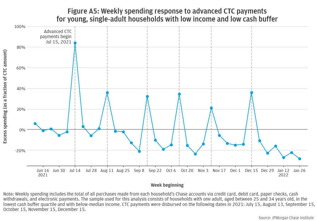
To assess how much these group-level differences in spending trends impacted regression results, we repeated our analysis on a subsample of our regression data. We held constant several key dimensions of differences between CTC recipient and non-recipient households with the goal of removing the underlying differences in spending trajectory. The subsample was restricted to young, single-adult households with low income and low cash buffer. This somewhat reduces the pre-existing differences in balances and EIP receipt and thus should reduce the variation in EIP-related deceleration between the CTC recipients and non-recipients. The resulting spending response shows a somewhat flattened trajectory, with monthly peaks and troughs at relatively constant levels, August through December (see Figure A5). Most analyses in this report focus on the overall regression sample, keeping in mind the source of this downward trend.
Figure A5: Weekly spending response to advanced CTC payments for young, single-adult households with low income and low cash buffer
Bastian, Jacob. 2022. “Investigating How a Permanent Child Tax Credit Expansion Would Affect Poverty and Employment.” Working paper. https://drive.google.com/file/d/1H5iNZZO_YFRIDz-3Tip4C-BpnD85bUjH/view
Corinth, Kevin, Bruce D. Meyer, Matthew Stadnicki, and Derek Wu. 2021. “The Anti-Poverty, Targeting, and Labor Supply Effects of the Proposed Child Tax Credit Expansion.” Becker Friedman Institute for Economics Working Paper No. 2021-115.
Farrell, Diana, Fiona Greig, and Amar Hamoudi. 2019. "Tax Time: How Families Manage Tax Refunds and Payments." JPMorgan Chase Institute. https://www.jpmorganchase.com/content/dam/jpmc/jpmorgan-chase-and-co/institute/pdf/institute-tax-time-report-full.pdf
Farrell, Diana, Fiona Greig, Chris Wheat, Max Liebeskind, Peter Ganong, Damon Jones, and Pascal Noel. 2020. “Racial Gaps in Financial Outcomes: Big Data Evidence.” JPMorgan Chase Institute. https://www.jpmorganchase.com/content/dam/jpmc/jpmorgan-chase-and-co/institute/pdf/institute-race-report.pdf
Karpman, Michael, Elaine Maag, Genevieve M. Kenney, and Douglas A. Wissoker. 2021. “Who Has Received Advance Child Tax Credit Payments, and How Were the Payments Used? Patterns by Race, Ethnicity, and Household Income in the July–September 2021 Household Pulse Survey.” Urban Institute. https://www.urban.org/sites/default/files/publication/105023/who-has-received-advance-ctc-payments-and-how-were-the-payments-used.pdf
Pilkauskas, Natasha and Patrick Cooney. 2021. “Receipt and Usage of Child Tax Credit Payments Among Low-Income Families: What We Know.” Poverty Solutions. https://sites.fordschool.umich.edu/poverty2021/files/2021/10/PovertySolutions-Child-Tax-Credit-Payments-PolicyBrief.pdf
Pilkauskas, Natasha, Katherine Michelmore, Nicole Kovski, and H. Luke Shaefer. 2022. “The Effects of Income on the Economic Wellbeing of Families with Low incomes: Evidence from the 2021 Expanded Tax Credit”. NBER Working Paper 30533. https://www.nber.org/system/files/working_papers/w30533/w30533.pdf
Wheat, Chris, and Erica Deadman. 2022. “Household Pulse through June 2022: Gains for most, but not all.” JPMorgan Chase Institute. https://www.jpmorganchase.com/insights/all-topics/financial-health-wealth-creation/household-pulse-cash-balances-through-june-2022
When the Child Tax Credit is non-refundable, parents do not receive the credit unless they have a tax liability to offset, so the CTC acts as a subsidy to labor income much like the Earned Income Tax Credit (EITC). Alternatively, the non-refundability of the credit could be viewed as a work requirement since most low-income parents’ income tax liability comes primarily from labor income. ARPA made the CTC fully refundable, removing this subsidy/work requirement effect and expanded the amount available per child. Using estimates of the labor supply effects of past benefits expansions, simulation studies find that a permanent CTC expansion would induce at least a moderate labor supply response (Bastian 2022; Corinth et al. 2021). However, these simulations still predict that the expanded CTC would significantly reduce child poverty even net of this negative labor supply response.
For example, President Biden’s proposed Build Back Better agenda includes extending the increased Child Tax Credit on an ongoing basis.
Families were automatically enrolled if the IRS processed their 2020 or 2019 tax return before the end of June 2021. Non-filers were also included if they had entered their information in 2020 to receive stimulus payments, or if they entered their information in 2021 via IRS non-filer tool:
https://www.irs.gov/credits-deductions/advance-child-tax-credit-payments-in-2021
We classify number of dependent children by the amount of EIP received by the household; see Data Asset section for additional discussion.
For details on how credit card transactions are handled, see the Dependent Variables discussion in the appendix.
The November payment has the lowest spending response due to including fewer post-CTC days to observe consumption activity. See the appendix for discussion of this and other caveats.
Non-durable spending includes cash withdrawals and spending on clothing, department stores, restaurants, transit, utilities, fuel, and groceries.
Durable spending includes spending on auto repair, home improvement, entertainment, and insurance.
Healthcare spending includes spending on drug stores, hospitals, and other healthcare.
The difference in response of Black households is statistically significant relative to Hispanic households (p-value 0.034) and White households (p-value 0.005).
Presence of dependent children in the CTC recipient group is inferred via receipt of all six advanced CTC payments, as described in the Data Asset section. Eligible families were proactively enrolled on the basis of dependent children indicated via tax filings or other non-filer tools; see CTC Background box for additional details. Absence of dependent children in the non-recipient group is inferred via the combination of zero advanced CTC payments and no dependent children indicated by the amount of EIP received by the household, as described in the Data Asset section. It is possible that some households in this group have added dependent children subsequent to the 2019 tax filings that determined those stimulus payments, and then proactively opted out of receiving advanced CTC payments. In other words, it is possible but rate that our non-recipient sample includes some households with dependent children.
So that each group gets its own set of βτ and δt, subgroup regressions use the following specification, where 𝟙g is a dummy variable for membership in group g:
yit=αi+δgt+∑g 1g (βgτ CTCi 1τ ) +εit
By definition, weights will be exactly 1 for all CTC recipient households.
We thank our research team, specifically Francesca Guiso, for her hard work and contribution to this research. Additionally, we thank Annabel Jouard and Robert Caldwell for their support. We are indebted to our internal partners and colleagues, who support delivery of our agenda in a myriad of ways, and acknowledge their contributions to each and all releases.
We are also grateful for the invaluable constructive feedback we received from external experts and partners. We are deeply grateful for their generosity of time, insight, and support.
We would like to acknowledge Jamie Dimon, CEO of JPMorgan Chase & Co., for his vision and leadership in establishing the Institute and enabling the ongoing research agenda. We remain deeply grateful to Peter Scher, Vice Chairman, Demetrios Marantis, Head of Corporate Responsibility, Heather Higginbottom, Head of Research & Policy, and others across the firm for the resources and support to pioneer a new approach to contribute to global economic analysis and insight.
This material is a product of JPMorgan Chase Institute and is provided to you solely for general information purposes. Unless otherwise specifically stated, any views or opinions expressed herein are solely those of the authors listed and may differ from the views and opinions expressed by J.P. Morgan Securities LLC (JPMS) Research Department or other departments or divisions of JPMorgan Chase & Co. or its affiliates. This material is not a product of the Research Department of JPMS. Information has been obtained from sources believed to be reliable, but JPMorgan Chase & Co. or its affiliates and/or subsidiaries (collectively J.P. Morgan) do not warrant its completeness or accuracy. Opinions and estimates constitute our judgment as of the date of this material and are subject to change without notice. No representation or warranty should be made with regard to any computations, graphs, tables, diagrams or commentary in this material, which is provided for illustration/reference purposes only. The data relied on for this report are based on past transactions and may not be indicative of future results. J.P. Morgan assumes no duty to update any information in this material in the event that such information changes. The opinion herein should not be construed as an individual recommendation for any particular client and is not intended as advice or recommendations of particular securities, financial instruments, or strategies for a particular client. This material does not constitute a solicitation or offer in any jurisdiction where such a solicitation is unlawful.
Wheat, Chris, Erica Deadman, Daniel M Sullivan. 2022. “How families used the advanced Child Tax Credit.” JPMorgan Chase Institute.
https://www.jpmorganchase.com/institute/all-topics/financial-health-wealth-creation/how-families-used-advanced-CTC
Authors

Chris Wheat
President, JPMorganChase Institute

Erica Deadman
Consumer Research Lead, JPMorganChase Institute

Daniel M. Sullivan
Consumer Research Director, JPMorganChase Institute