
Figure 1: Cash buffers and gaps across income groups were stable before the pandemic-era fluctuations.
Latest news

An Ohio-based company is protecting first responders around the world
With support from JPMorganChase, Fire-Dex is providing protective equipment to firefighters in 100 countries and all 50 states.
Learn moreLatest news

Veteran’s Unconventional Path to Landing her Dream Job in Tech
U.S. Army Veteran Ashley Wigfall transitioned to a civilian role and charted her path to technologist through mentorship and skills training at the JPMorgan Chase tech hub in Plano, Texas.
Learn more
Findings
Introduction
Cash balances are a linchpin of household financial health. Maintaining a sufficient level of liquidity—which varies with spending needs—allows households to manage spending through short-run changes to income. Over time, savings in the form of cash can also be used for large expenditures or wealth-building investments. The dynamics of checking account balances therefore reflect both consequences of external shocks affecting consumers—e.g., job loss, fiscal stimulus, or unexpected expenses—as well decisions of when and how to save.
COVID-19 brought economic volatility that led to historic swings in the savings rate from a record high in 2020 to very low levels last year before rising steadily in recent months, reflected in trends in cash balances seen in the most recent JPMorgan Chase Institute Household Pulse report. In addition to measuring cash liquidity over a longer time horizon, this report analyzes within-household cash management behavior to help make sense of recent fluctuations. We use a sample of de-identified data covering 19 million individuals from 2008 through early 2023.
Our focus is on cash buffers (liquid balances scaled to expenses), interpreted as the amount of time a person could continue their rate of spending without receiving inflows or accessing new credit. The research questions we target in this report are:
A central finding of this report is the relative stability in cash buffers for over a decade prior to the surge in balances during the pandemic. From 2008 to 2019—a period over which the unemployment rate swung from as high as 10 percent to under 4 percent—median cash buffers stayed within a range of just a few days’ worth of spending.1 While we also find that many individuals frequently experience large swings in liquidity, these idiosyncratic surges and dips do not normally last very long. This is because individuals tend to spend in excess of income when cash buffers are temporarily elevated and vice versa.2
The ongoing decline in the stock of cash balances that were built up in the pandemic is qualitatively consistent with pre-pandemic patterns, although the drawdown has been somewhat slower than usual, according to our estimates.
We organize the analysis around four findings:
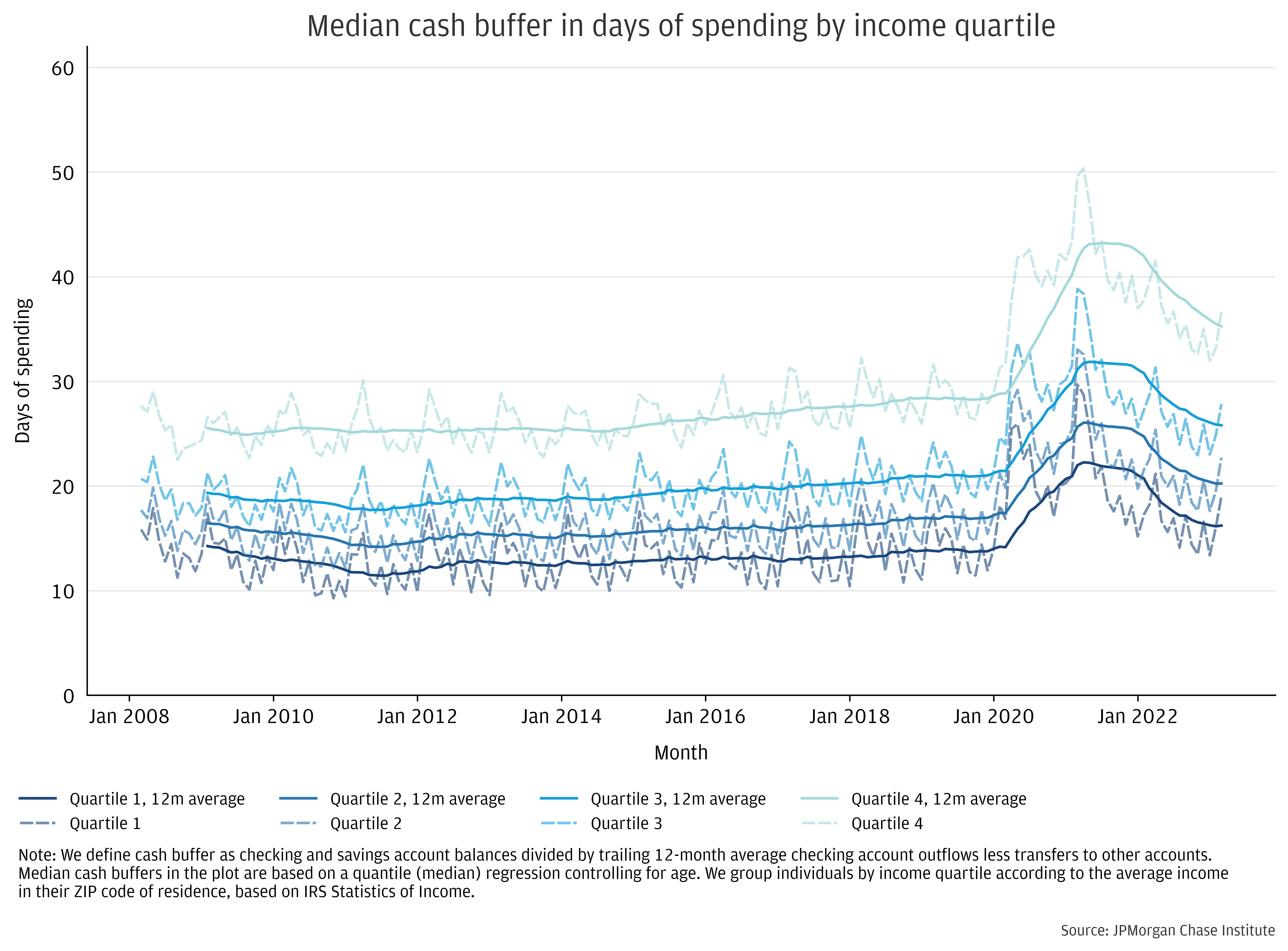
Individuals with lower average incomes tend to hold lower amounts in liquid balances relative to spending, otherwise referred to throughout as cash buffer.3 Over our sample window from 2008 through early 2023, median cash buffers for the bottom income quartile averaged about half that of the top income quartile. Both the overall level of median cash buffers and gaps across income quartiles were roughly stable prior to the pandemic.
COVID-19 led to a temporary decline in spending starting in March 2020 followed by a rise in income growth fueled by fiscal stimulus, leading to a surge in cash buffers that was more pronounced in percentage terms for lower-income individuals.4 These effects on income had largely dissipated by the end of last year for most people while spending has remained robust, on balance, resulting in the current trend of declining cash liquidity towards the levels observed from 2008 to 2019 across groups, albeit at somewhat varying speeds. In Finding 4 we leverage the dynamics of individual-level cash buffers to help make sense of the trend of “normalizing” household liquidity.
Figure 1: Cash buffers and gaps across income groups were stable before the pandemic-era fluctuations.
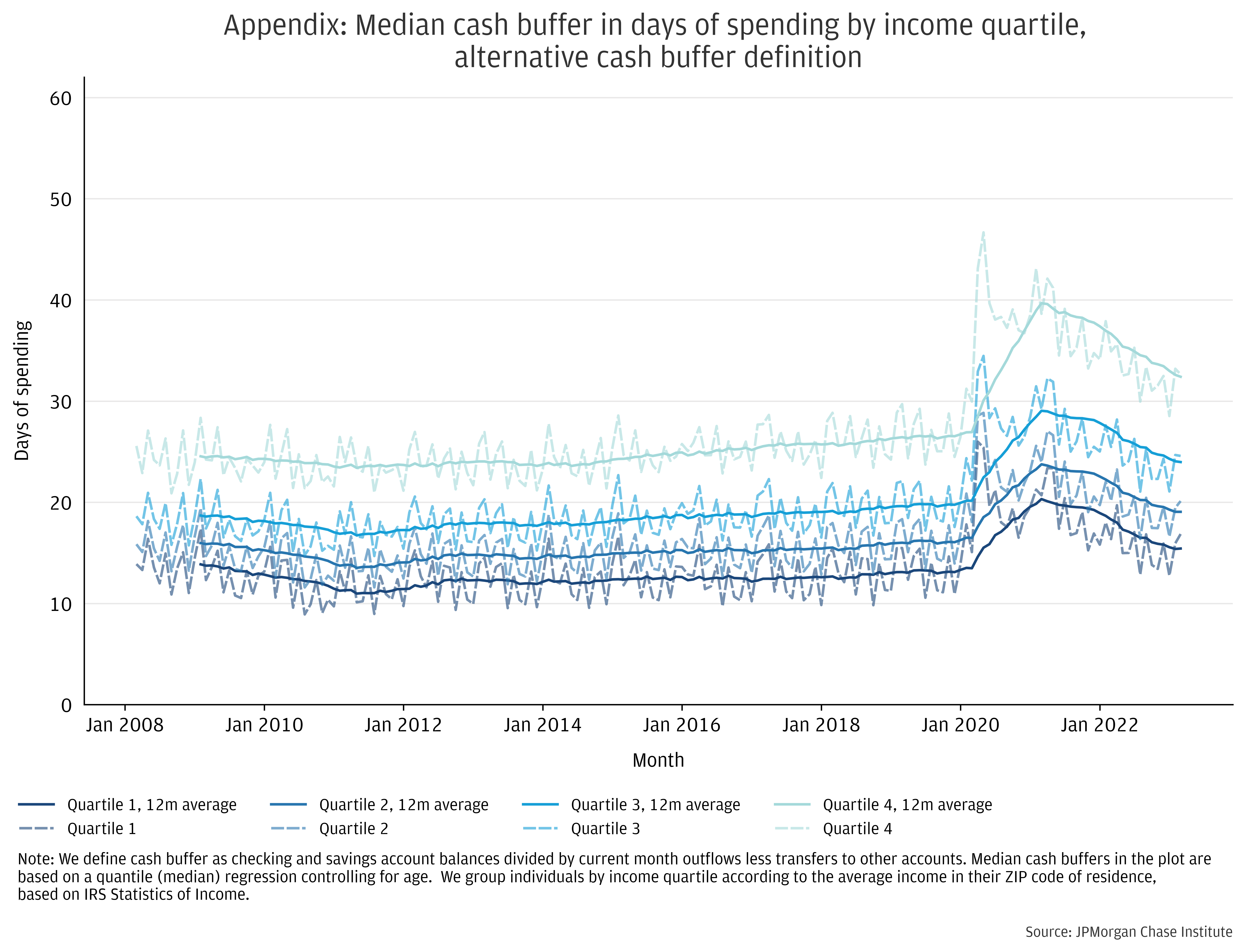
We track the median level of cash buffers using a regression-based framework. This helps minimize the effect of changing composition of our sample over time, but it means that our figures for median cash buffer are ‘estimates,’ as opposed to directly measured median values. Appendix A provides details on the approach. An assumption we make in Figure 1 is that the relevant rate of a person’s spending is their trailing 12-months’ median outflows excluding account transfers. We show an analogue to Figure 1 that instead computes cash buffer by dividing liquid balances by the current month’s outflows excluding transfers. Due to sharp changes in spending in 2020 and 2021—e.g., declining around the onset of the pandemic, then surging in the wake of fiscal stimulus—the contours of cash buffers over that period differ somewhat across the two methods for cash buffers. Moreover, since both spending and cash balances exhibit seasonality, the calendar year pattern of cash buffers also changes with the methodology.
Black and Hispanic individuals experienced relative income gains as the unemployment rate reached historically low levels in the years preceding the pandemic.5 Moreover, fiscal supports provided a more pronounced boost to Black and Hispanic individuals’ incomes during 2020 and 2021. Despite relative income gains in recent years, racial disparities in cash buffers in our data did not diminish.6 To analyze these differences, we rely on a subsample of 1.4 million individuals for whom we have self-reported race data.7
Figure 2: Racial gaps in cash buffers persist, despite relative income gains of Black and Hispanic individuals in recent years.
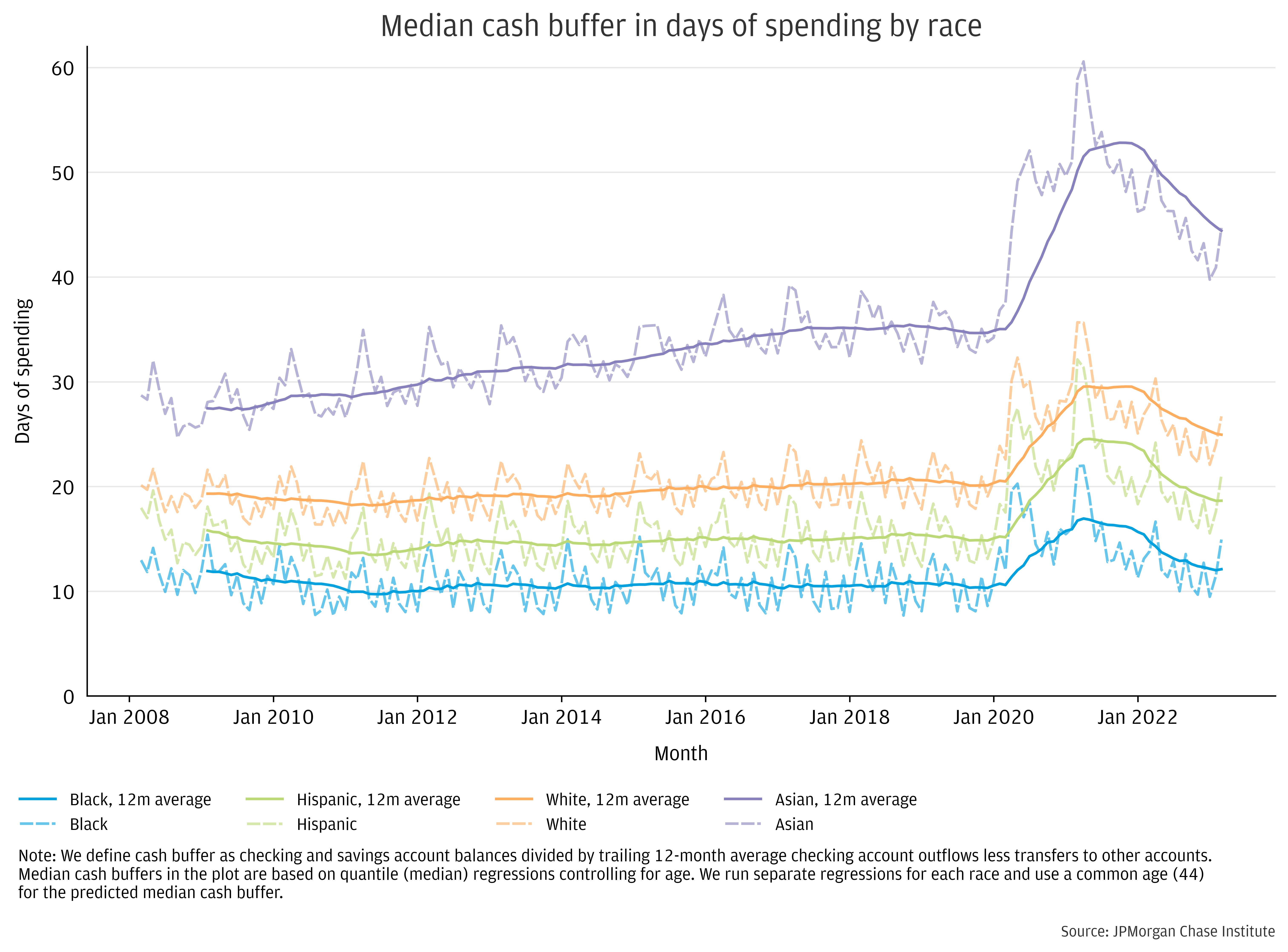
Early in the recovery from the Great Recession, Black and Hispanic individuals’ income growth was similar to that of White individuals.8 As the labor market subsequently tightened, income growth for Black and Hispanic individuals began exceeding both Asian and White individuals by about 1 percentage point per year, over from 2017 to 2019. These relative gains extended during 2020 and 2021—due to the impact of Unemployment Insurance and Economic Impact Payments—but the boost to incomes was short-lived.
Liquidity by race directionally tracked income growth in the pandemic. Black and Hispanic individuals saw the largest percent rise in cash buffers at the pandemic peak relative to the 2019 average. However, those liquidity gains were smaller when measured in dollars relative to White and Asian individuals, due to Black and Hispanic individuals’ lower baseline level of liquidity. Moreover, Black individuals experienced a more rapid reversal of cash buffer gains, leaving a somewhat larger range separating racial groups as of early 2023 compared to the average over the 2010s.9
Even in normal economic conditions, month-to-month changes in individual incomes can be highly volatile, frequently leading to large shifts in cash balances.10 This means that a high degree of individual-level variability underlies the relative stability in median balances across the economy in pre-pandemic data. To shed light on individuals’ experience managing their liquidity, here we examine individual-level variation, leveraging statistics from a subsample of 12 million individuals with at least 5 years of active account history.11 To avoid excess influence of the pandemic, we focus on the period from the Great Recession and the pandemic, 2008 to 2019, for Finding 3.
To quantify volatility in cash buffers, we use two measures that scale month-to-month fluctuations to a person’s usual level of balances. Figure 3 shows the median of these metrics by income quartile. The first measure is the standard deviation of a person’s cash buffer scaled by their average level of cash buffer.12 Another metric based on medians—the scaled median deviation from median cash buffer—provides a view of volatility less influenced by outliers.
Figure 3: Volatility in cash buffers over time is substantial at the individual level and is somewhat higher—when scaled to a person’s level of liquidity—for lower-income individuals.
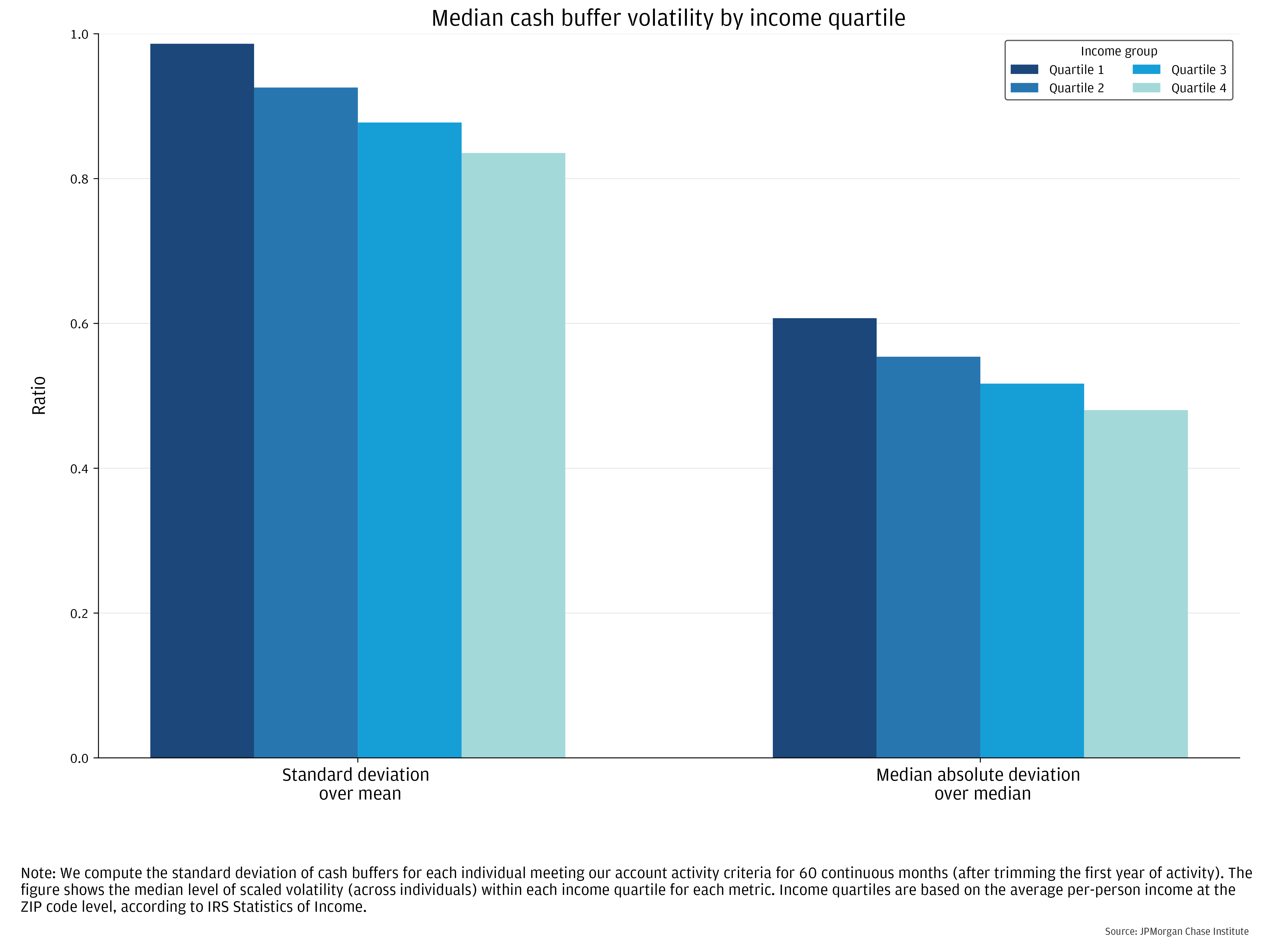
Both metrics depicted in Figure 3 imply substantial variation over time in household liquidity. Using the first measure, typical variation in cash buffers is equal to 80 to 100 percent of a person’s usual cash buffer level. The influence of large, but infrequent, shocks to cash balances has a more substantial effect on the first measure, which is somewhat higher than the second metric.13 For a sense of scale, the 12-month average level of median cash buffers moved up to a peak of 22 days from 13 (70 percent increase) for the first income quartile and to 44 from 28 (60 percent increase) for the top quartile, coinciding with the largest increase in the personal savings rate since World War II. From this perspective, the typical level of variation in liquidity is substantial at the individual level.
Spikes in liquidity provide opportunities for wealth-building as well as spending to satisfy unmet needs. To analyze differential responses to increases in cash buffers due to positive income shocks, we provide a supplemental analysis of how people use funds in the month of a large increase in income in Appendix B. When filtering to events in which monthly income was between 2.5 to 12 times a person’s trailing average level of income, less than half of the abnormal inflow remain in individual’s checking accounts by the end of the month it is received, on average, across income quartiles. Differences by income group in the deployment of funds are consistent with prior findings of the higher tendency of lower income individuals to consume out of temporary gains, while those with higher incomes are more likely to transfer excess funds to savings vehicles like investment accounts.14
On the other hand, dips in cash buffers can indicate financial distress, although the presence of liquid assets not captured in our data may dampen such an interpretation. Figure 4 shows the share of individuals that have less than 7 days’ worth of spending in liquid balances along with the portion of those people with investment accounts to provide a perspective on why such metrics should be interpreted with care.15 Because the highest income quartile is the most likely to have other liquid assets outside of our data set, looking solely at cash buffer metrics understates disparities in financial vulnerability across the income distribution.
Figure 4: Individuals with lower average incomes are more likely to have under one week’s worth of spending in liquid balances and are less likely to have stores of liquidity outside of cash-like accounts.
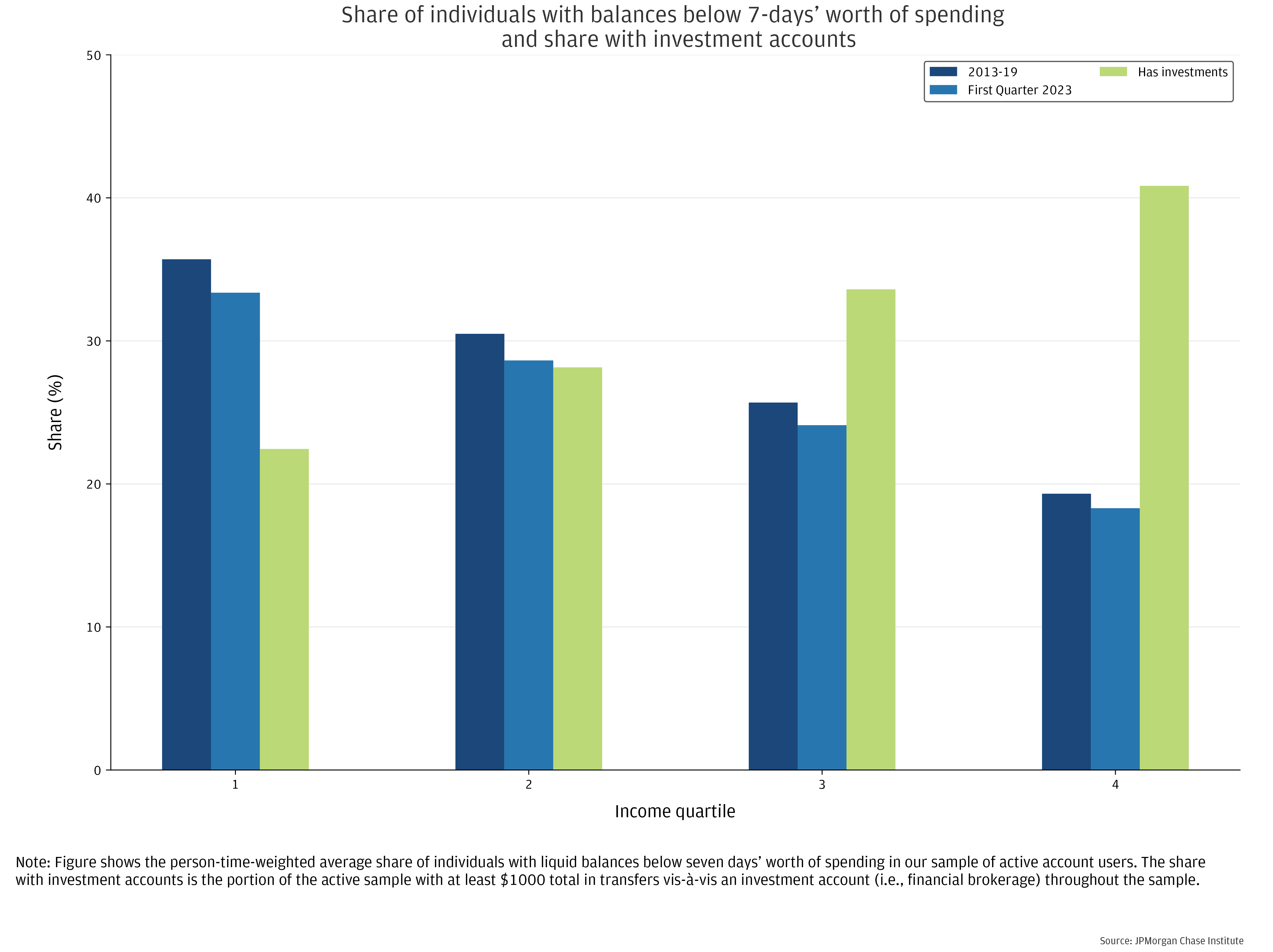
Individuals in the first income quartile are almost twice as likely to have less than 7 days’ worth of spending in liquid balances relative to those in the top income quartile. Even though cash buffers have been falling from their peak in 2021, the share of individuals with under 7 days’ worth of spending in cash-like accounts in our data remained modestly below pre-pandemic standards through the first quarter of this year. We do not view these metrics as precise indicators of the share of individuals facing financial distress; as noted earlier, these figures almost certainly underestimate disparities, due to the greater share of high-income individuals that have other stores of liquid wealth not captured in these data.
To help make sense of the recent decline in median cash buffers towards pre-pandemic norms, we look at individual-level data on the evolution of cash buffers when balances deviate from normal. Informed by the pre-pandemic stability in cash buffers, our hypothesis is that individuals adjust spending and other behavior to manage their cash buffer to some typical level following shocks. We find a consistent pattern of individuals managing towards levels of cash buffer they maintained previously. When an individual’s cash buffer is abnormally high—i.e., above their trailing baseline—they spend down or transfer excess liquidity and vice versa. Outside of the savings surge of 2020-21, the pace of individual-level normalization has been surprisingly consistent with pre-pandemic experience.
Figure 5 depicts how individuals’ savings behavior (defined as changes in cash balances, scaled to spending) varies depending on a person’s level of cash buffer relative to a prior norm. Here, we use a 36-month lagged value of a person’s cash buffer as the baseline. In addition to helping remove seasonality, this view allows for a consistent methodology for comparing liquidity normalization observed over the course of last year against prior periods. Before COVID, the median individual reached a savings rate of zero (in terms of changes in cash balances) when they had one more cash buffer day than they had 36 months prior. In the pandemic years of 2020 and 2021, individuals had shifted their savings behavior—individuals with a buffer of about two and a half days were neither increasing nor decreasing their cash balances at the median. By 2022, individuals were reaching a stable level of cash buffers a single day above the level observed three years prior, as they had before the pandemic. At a cash buffer level one week above baseline (+7 days on the plot), the median savings rate is -8 percent, implying a decline in excess cash buffer of 2 days. This pace of declines moderates as individuals approach their prior “normal.”
Figure 5: Cash balances evolve asymmetrically, as building liquidity usually takes longer than spending it down.
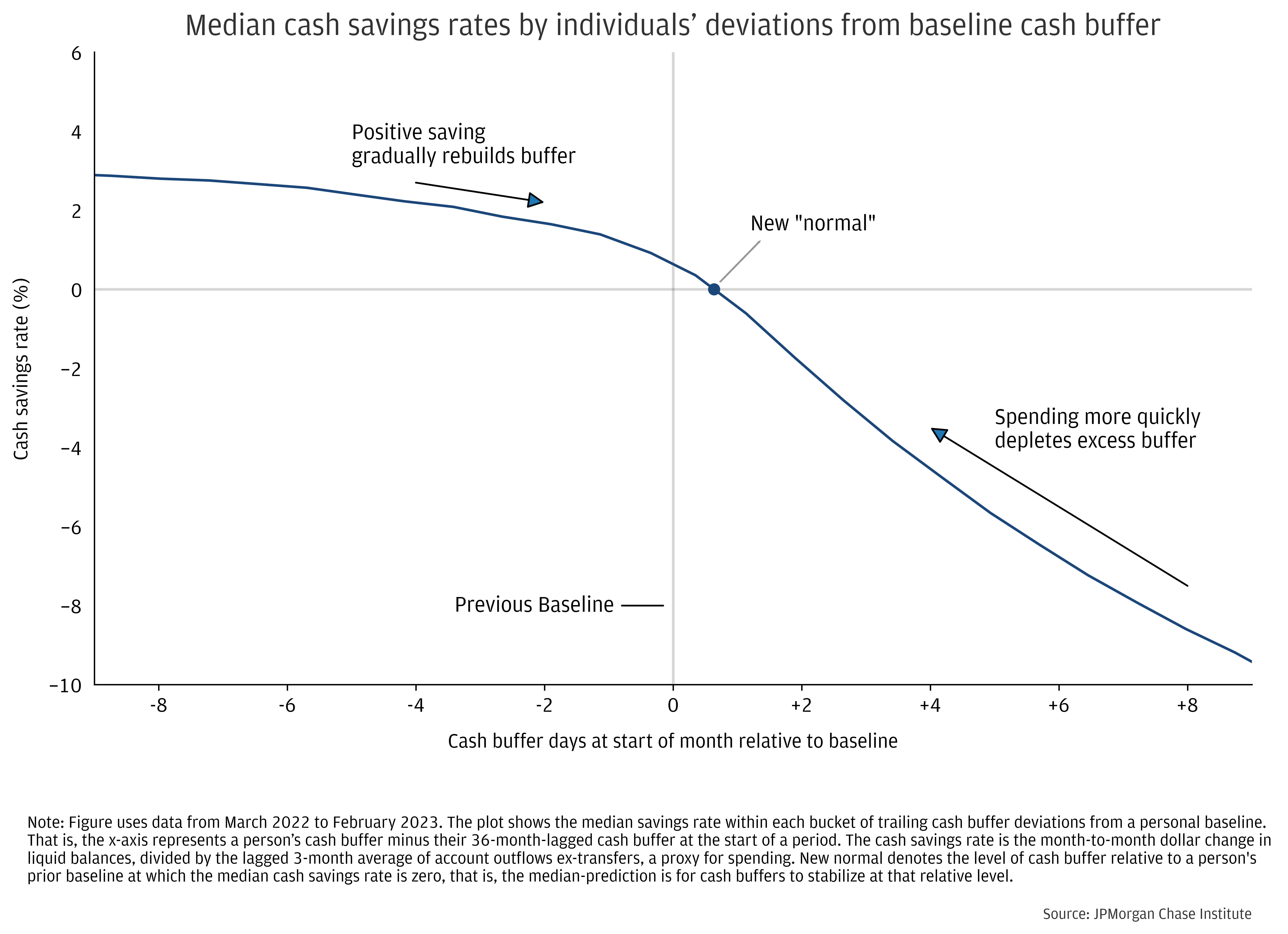
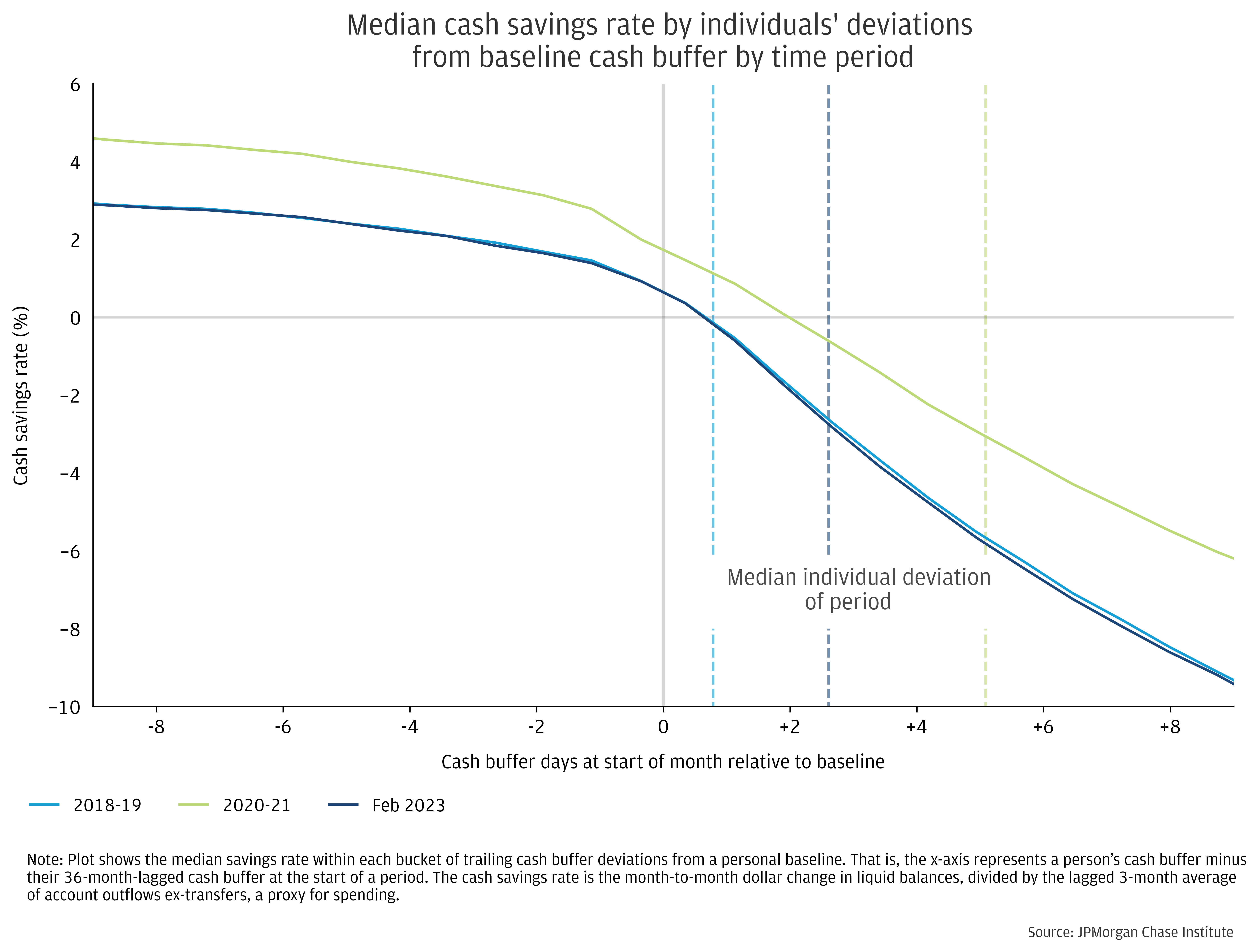
Figure 6: The dynamics of individuals’ cash buffers since early 2022 has closely followed the pattern seen in general variation in liquidity observed prior to the pandemic.
How we quantify a person’s baseline liquidity and cash savings rate
The analysis underlying Figures 5 through 7 is based on three elements: (1) a person’s cash buffer; (2) an estimate of a person’s past “normal” cash buffer; and (3) a savings rate out of take-home pay. We use the same cash buffer concept used earlier in this report. For the “normal” cash buffer estimate, we take a person’s cash buffer 36 month’s prior. This allows a view of normalization to a pre-pandemic baseline in data through early 2023. Our results do not shift substantially when altering the lag length or using a trailing window for baseline cash buffer. For someone’s liquidity deviation from normal, we take the difference between the current cash buffer and that baseline. Finally, the savings rate proxy is the next month’s dollar change in cash balances divided by the trailing 12-month median level of outflows ex-transfers.
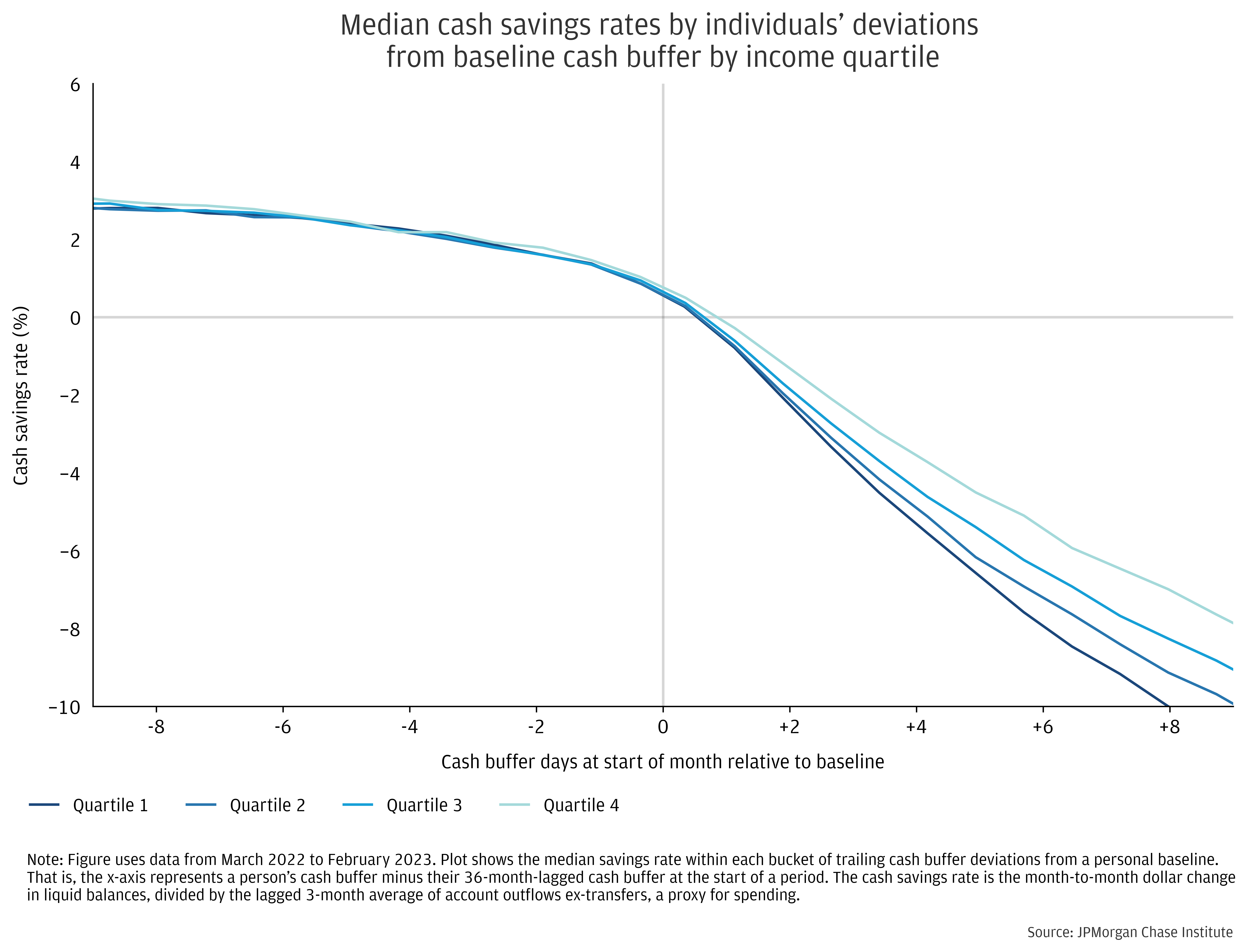
Liquidity normalization differs somewhat across the income spectrum. Figure 7 depicts the process of cash buffer adjustment by income quartile. While patterns—mean reversion and asymmetry—are qualitatively consistent across groups, we see notable differences in magnitudes that inform how different individuals respond to shocks. When cash balances are 10-days below a personal baseline, the median individual in the fourth income quartile builds buffer days by about the same pace as the lowest quartile. However, reductions of excess cash buffers occur more quickly for lower income individuals. For a cash buffer level 10 days above baseline, the median individual in the top income quartile reduces their cash holdings by 7 percent of income, compared to 10 percent for the bottom quartile.
Figure 7: Cash buffers decline more quickly for lower income individuals when liquidity is above normal.
While Figures 5 to 7 depict the pattern of cash buffers, the actual transactions that influence those dynamics—e.g., spending and account transfers—contain additional information about how and why household liquidity changes over time. In Appendix B we look at significant income shocks and how they are diffused across liquid balances, spending, and savings or transfers. In a result that informs the dynamics underlying cash buffer normalization shown here—we find that higher income individuals adjust liquidity following a positive income shock by increasing savings-related flows (like transferring funds to investment accounts) and experience comparatively less of an increase in spending.
Conclusion
The pre-pandemic stability in household liquidity metrics described in this report implies that a relatively wide range of economic factors can lead to the same approximate level of cash balances, when scaled to expenses. Moreover, we observed relatively little net change over time in the liquidity gaps across income quartiles and by race over the sample. By contrast, economic volatility during the pandemic led to historic swings in aggregate measures of liquidity, with median cash buffers almost doubling by the April 2021 peak in the measure. Since then, household liquidity has been normalizing, as cash balances have been receding and nominal expenses rising.
We zoom in on individual-level experiences of shocks to make sense of recent trends. During the savings normalization process in 2022 through early 2023, individual liquidity management patterns have been similar to earlier periods. On balance, people tend to manage their balances towards a level of expense coverage and save or spend their way back to prior averages following shocks. The slowing of the declines in liquidity observed in the Household Pulse—and the faster pace of normalization for lower income individuals—is a consistent pattern seen across varying environments over the past decade with little variation outside of the height of the pandemic. Even so the present economic environment has unique features relevant for household liquidity management—including higher short-term interest rates, changing investment trends, and potential new precautionary savings motives.16 These factors could lead individuals to choose either a higher level of cash buffer—perhaps to guard against uncertainty in inflation or fears about job security in a potential recession—or a lower level—to extract higher interest rates in products other than cash deposits, such as bonds or certificates of deposit.
Implications
This report provides insights into household liquidity management relevant for macroeconomic policymakers as well as the design of microeconomic policies, including asset limits. In terms of the macroeconomic outlook, our findings provide a perspective on how the pandemic wave of savings may influence consumer demand in the coming quarters. While no recent U.S. precedent exists for an aggregate savings shock of the magnitude seen in 2020 and 2021, patterns documented in this report from idiosyncratic experiences demonstrate a strong tendency for even substantial shocks to dissipate and for cash buffers to gravitate towards the pre-shock level, all else equal. The pattern seen in cash buffers—both in the aggregate and individual-levels—since the pandemic peak is consistent with pre-pandemic behavior.
Gauging financial health implications of individual-level volatility in cash buffers is challenging. Both the level and variability in cash buffers can be the result of smoothing consumption amid income volatility, which is usually a good sign for well-being. Meanwhile, costly decisions (from a quality-of-life perspective) like foregoing spending to preserve cash would mask potential damage to people’s lives.17
Indeed, households’ preferences and decisions appear to influence liquidity levels strongly, as do events outside of their control. Individuals with lower liquidity tend to spend more out of programs like stimulus payments and safety net programs like Unemployment Insurance. The tendency to consume out of programs may suggest the attractiveness of targeting fiscal support based on liquidity. However, doing so could lead individuals to choose a lower level of cash liquidity, i.e., incenting behavior leading to financial vulnerability. Moreover, due to considerable volatility (at the individual level) in cash buffers, a person approaching a policy threshold may fall in and out of eligibility, with little connection to a steady underlying need. In cases in which policymakers see value in asset limit testing, our research suggests that the dollar values should be scaled to a proportion of consumption spending and emergency savings needs. This would help calibrate the delivery of government support to the level of financial risk facing a family and keeps pace with inflation over time.
Appendix A: How we measure median cash buffers over time
Due to potential changes in median liquidity resulting from shifts in the Chase footprint over time, we use a statistical framework that controls for age and other variables. The following equation represents our regression-based methodology. The outcome variable, yit, is the amount of a person i’s liquid balances in time t, relative to a measure of spending. We estimate the regression separately for individuals in each income group, g. The regression controls for age (only individuals between 25 and 70 are included), whether a person was in our data prior to 2009, Earlyi (significant changes in sample composition occurred at that point), and a month fixed effect, δ( gt), which drives the dynamics of the time series.
yit= βg ageit+Earlyi+δ( gt)+eit , for individuals i in income group g.
As opposed to a standard ordinary least squares regression—which provides an estimate for average liquidity—we focus on medians, relying on a quantile regression. This method reduces the impact of outliers and better tracks outcomes prevailing for the typical individual.18 The resulting estimates provide the expected median cash buffer for each income group, holding variables other than time constant. Coefficients for each month and income group in our sample allow for flexible variation over time. For Figures 1 and 2, we use a person 44 years old and a value of 50 percent for ‘Early.’
In Figure 1 of this report, the rate of spending used to compute a cash buffer is a person’s median monthly level of account outflows less transfers over the prior 12 months. Below in Figure A, we substitute a measure that divides liquid balances by the current month’s level of outflows excluding account transfers. While the overall level and dynamics are similar, the timing of the peak of cash buffers during the pandemic is in 2020 as opposed to the peaks seen in Figure 1, which came in 2021.
Figure A: Using a different definition of cash buffer changes the seasonal pattern and timing of the pandemic peak in cash buffers somewhat.
Appendix B: Liquidity events
Individuals tend to manage cash buffers back to a preferred level by a range of mechanisms: adjusting spending, using or paying down credit balances, and transferring funds vis-à-vis longer-term savings accounts (e.g., investment accounts). To examine one aspect of adjustment, we study the response of individuals to large income shocks: defined by a month in which inflows excluding transfers is between 2.5 to 12 times the trailing year’s average. Given we’re interested here in general behavior, we limit the event sample to pre-pandemic data.
In this framework, we find that the role of savings-related transfers is greater for higher income individuals, whereas spending increases drive a relatively greater share of the declines in checking account balances for those with lower incomes. Figure A documents the flow of money to different destinations in the month of the shock when individuals disburse the majority of the income shock. The average change in balances is somewhat higher for the top income quartile—consistent with Figure 6, which shows a more tempered cash depletion response for higher income individuals when balances are above normal. Even so, higher income individuals transfer funds out of liquid balance accounts—to, for example, investment or money fund accounts—and pay off credit card balances, relative to lower-income individuals, who conduct more direct spending out of their liquid balance accounts (seen in the ‘Spending change’ category of Figure B).
Figure B: Higher income individuals are more likely to save—including by paying off debt—out of significant income gains.
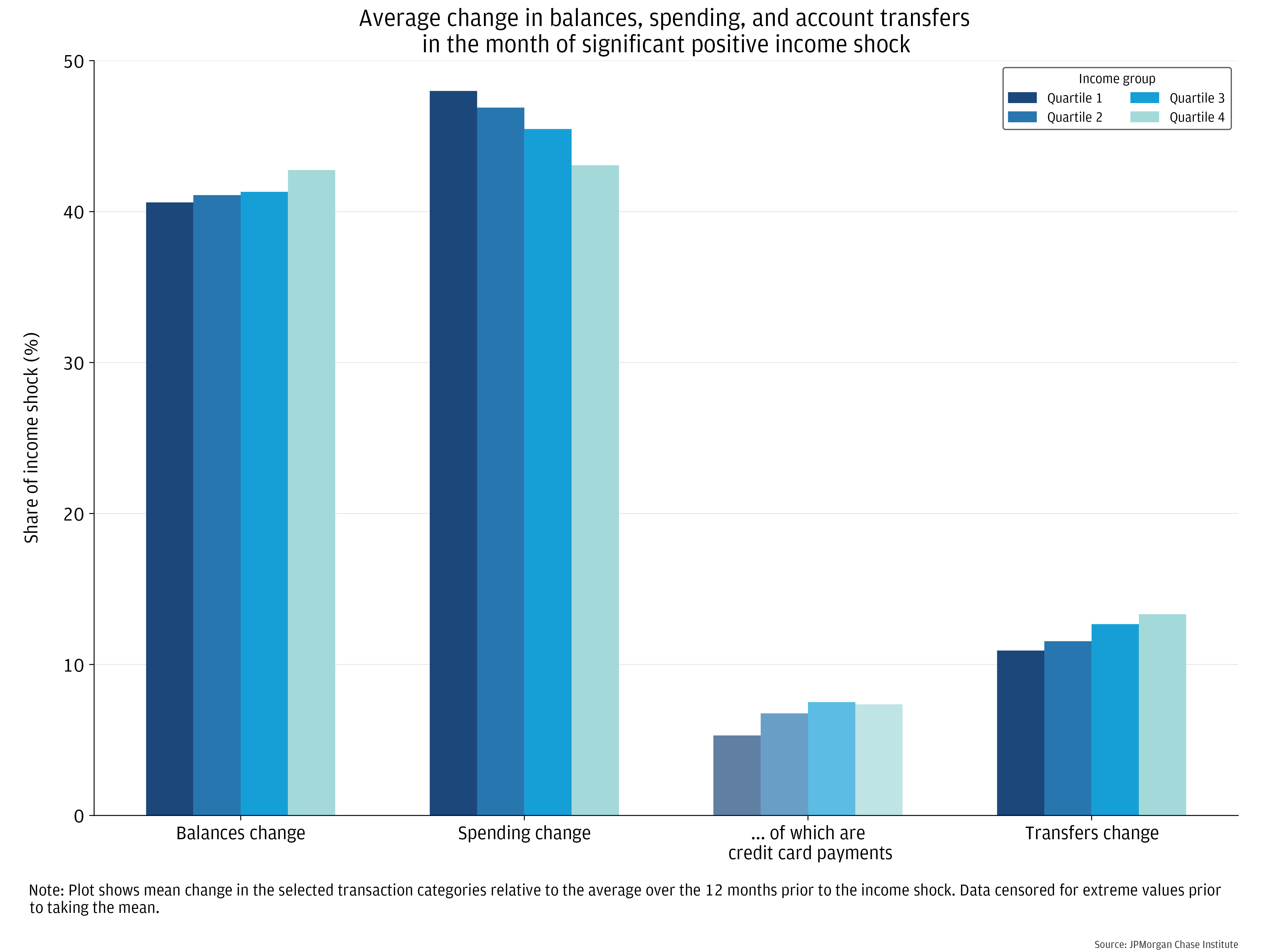
The greater share of potential savings-related transactions—i.e., transfers and higher payments to credit cards—for higher income individuals shown here is consistent with prior academic and Institute analyses that find a higher marginal propensity to consume for lower income households. The role of transfers to savings vehicles and paying down debt may inform an understanding of the lasting changes to household balance sheets from the pandemic savings surge, notwithstanding potential normalization in liquidity metrics like cash buffers.
After smoothing over seasonal variation, such as fluctuations due to tax refunds.
In addition to adjusting spending, individuals manage liquidity in cash deposits by using transfers vis-à-vis other accounts, such as investment brokerage accounts, or allow credit card balances to fluctuate.
Data from the Federal Reserve’s Survey of Consumer Finances indicate that this is true even though households with lower incomes tend to hold a larger share of their wealth in the form of cash accounts (see, for example, Figure 6 of Wealth Inequality and the Racial Wealth Gap, FEDS Note, October 2021).
Institute Cash Pulse reports document these trends, although those analyses centered on cash balances indexed to pre-pandemic levels, rather than cash buffers (cash balances relative to spending) as in this report.
See Institute report Racial Income Inequality Dynamics (2022).
Progress on closing racial wealth gaps has been slow—as described in the recent paper, “Wealth of Two Nations: The U.S. Racial Wealth Gap, 1860-2020” by Ellora Derenoncourt, Chi Hyun Kim, Moritz Kuhn & Moritz Schularick (2022). Meanwhile the Survey of Consumer Finance provides a clear picture that wealth gaps are notably wider than income disparities and racial wealth inequality did not change substantially from 2016 to 2019 (Dutta et al., 2020).
Self-identified demographic data was obtained in 2021 from a third party for the JPMorgan Chase Institute to conduct economic research examining financial outcomes by race, ethnicity, and gender. The demographic data was matched to internal banking records using encrypted quasi-identifiers. This de-identified file that contains banking records and demographics is only available to the JPMorgan Chase Institute.
See Institute report Racial Income Inequality Dynamics (2022).
The average difference between Black and White individuals’ cash buffer days was 9 days (19.5 to 10.5) from 2010 to 2019 and rose to 12 days for the three months ending March 2023.
Cash balance changes arise from the difference between account inflows and outflows. Holding account transfers constant, this means that cash balances essentially track relative trends in income and spending.
In tracking changes over time in cash buffers, we require an individual to have 60 continuous months of activity and throw out the first 12 to avoid distortions related to shifting economic activity across accounts. As in the earlier Findings, we measure cash buffer as an individual’s liquid balances with Chase divided by trailing 12-month trailing median checking account outflows less transfers.
This statistic is known as the coefficient of variation.
The distribution of monthly changes in both incomes and cash balances is substantially positively skewed.
For a recent example, see Institute research on spending out of the advanced Child Tax Credit in 2021.
Funds held in financial investments, like taxable (i.e., non-retirement) brokerages accounts, are fairly liquid in the sense that sales of securities can be converted into cash with relative ease. However, they do not fit the definition of cash liquidity used as the primary indicator of cash buffers in this report.
The recency of a high degree of economic volatility could lead to more precautionary savings in liquid assets. Meanwhile higher short-term interest rates, theoretically, could draw cash out of low (or no return) liquidity into investments with higher returns. A separate factor is the precedent set by a historically large fiscal intervention in the form of cash transfers. If individuals expect a repeat of such policy action, it could unwind an incentive for precautionary saving.
A related conclusion seen in prior academic and Institute papers is that lower-income and lower-liquidity households tend to have a higher sensitivity of spending to income shocks. The closer connection between spending and income variation would tend to suppress variation in cash balances, all else equal. In this sense, welfare costs of cash buffer variation are likely more pronounced for those with low incomes and liquid balances than a straight read of Figure 4.
For discussion of quantile regression see, Koenker and Hallock (2001). Koenker, Roger, and Kevin F. Hallock. 2001. "Quantile Regression." Journal of Economic Perspectives, 15 (4): 143-156.
Bhutta, Neil, Andrew C. Chang, Lisa J. Dettling, and Joanne W. Hsu (2020). "Disparities in Wealth by Race and Ethnicity in the 2019 Survey of Consumer Finances," FEDS Notes. Washington: Board of Governors of the Federal Reserve System, September 28, 2020, https://doi.org/10.17016/2380-7172.2797.
Derenoncourt, Ellora, Chi Hyun Kim, Moritz Kuhn, and Moritz Schularick. “Wealth of Two Nations: The U.S. Racial Wealth Gap, 1860-2020.” IDEAS Working Paper Series from RePEc, 2022.
We thank our research team, especially Guillaume Kasten-Sportes, Khushboo Chougule, Melissa O’Brien, and Edward Biggs for their contributions to the analysis. We also thank Robert Caldwell and Annabel Jouard for their support. We are indebted to our internal partners and colleagues, who support delivery of our agenda in a myriad of ways and acknowledge their contributions to each and all releases.
We would like to acknowledge Jamie Dimon, CEO of JPMorgan Chase & Co., for his vision and leadership in establishing the Institute and enabling the ongoing research agenda. We remain deeply grateful to Peter Scher, Vice Chairman, Tim Berry, Head of Corporate Responsibility, Heather Higginbottom, Head of Research & Policy, and others across the firm for the resources and support to pioneer a new approach to contribute to global economic analysis and insight.
This material is a product of JPMorgan Chase Institute and is provided to you solely for general information purposes. Unless otherwise specifically stated, any views or opinions expressed herein are solely those of the authors listed and may differ from the views and opinions expressed by J.P. Morgan Securities LLC (JPMS) Research Department or other departments or divisions of JPMorgan Chase & Co. or its affiliates. This material is not a product of the Research Department of JPMS. Information has been obtained from sources believed to be reliable, but JPMorgan Chase & Co. or its affiliates and/or subsidiaries (collectively J.P. Morgan) do not warrant its completeness or accuracy. Opinions and estimates constitute our judgment as of the date of this material and are subject to change without notice. No representation or warranty should be made with regard to any computations, graphs, tables, diagrams or commentary in this material, which is provided for illustration/reference purposes only. The data relied on for this report are based on past transactions and may not be indicative of future results. J.P. Morgan assumes no duty to update any information in this material in the event that such information changes. The opinion herein should not be construed as an individual recommendation for any particular client and is not intended as advice or recommendations of particular securities, financial instruments, or strategies for a particular client. This material does not constitute a solicitation or offer in any jurisdiction where such a solicitation is unlawful.
Wheat, Chris, George Eckerd. 2023. “Household Cash Buffer Management from the Great Recession through COVID-19.” JPMorgan Chase Institute. https://www.jpmorganchase.com/insights/all-topics/financial-health-wealth-creation/household-cash-buffer-management-from-the-great-recession-through-covid-19
Authors

Chris Wheat
President, JPMorganChase Institute

George Eckerd
Wealth and Markets Research Director, JPMorganChase Institute